Question

4. Consider two firms with identical fixed costs, but different variable costs (for example, one firm has access to cheaper inputs or is located closer to the point of sale than the other): c. (g) = 625+q and MC,-1 and G (9)-625 + 492 and MC,-89 Find average total, average fixed and average variable cost functions for the two firms a) b) Find the minimum efficient scale of each firm average cost at MES (Hint: Use MC ATC rule). Which firm will be able to achieve lower average cost point?

Answer 1

a).

Now, the cost functions of two firms are given by, “C1 = 625 + q” and “C2 = 625 + 4q^2”. So, the “Average Total Cost” is given by, “ATC = C/q.

=> ATC1 = (625+q)/q = 625/q + 1, => ATC1 = 1 + 625/q. Now, ATC2 = (625 + 4q^2)/q.

=> ATC2 = 4q + 625/q.

Now, the AFC for both the firms are given by, “AFC1 = 625/q” and “AFC2 = 625/q”. Since, the “FC” for both the firms are same, => AFC for both the firms are also same.

Similarly, AVC for both the firms are given by, “AVC = VC/q”, => AVC1 = VC1/q = q/q = 1 =AVC1.

For 2^nd firm it is given by, “AVC2 = VC2/q = 4q^2/q = 4*q = AVC2.

b).

Now, for “firm 1” the “ATC” and “MC” are given by.

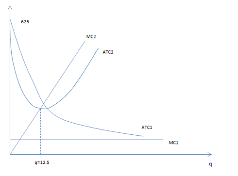
=> ATC1 = 1 + 625/q, => ATC is down ward sloping and MC = 1, => MC is constant at “1”. So, here “ATC” is asymptotic to “MC” at “MC = ATC”. So, when “q” is infinitely large “625/q” is close to “zero” and “ATC” is equal to “MC”.

Now, for the “firm2” the “ATC2 = 4q + 625/q” and “MC=8q”, => at “ATC2=MC2”.

=> 4q + 625/q = 8q, => 4q = 625/q, => 4q^2 = 625, => q^2 = 625/4, => q = 25/2 = 12.5. Now, for “firm 2” the minimum efficient scale is given by, “q=12.5”. So, at “q=12.5” the corresponding “ATC” and “MC” are given by, “100”.

c).

Consider the following fig shows the “ATC” and “MC” for both the firms.

d).

Here “type 1” will be more competitive compare to “type 2”. Since “type 1” having less “MC=1 < MC2=100” compare to “type 2” and having larger output or scale.