
Choose one answer for the purple blanks, answer number for orange blanks
Thanks!
Homework Answers
Engine size data has approximately same values of Mean, Median and Mode, So Engine size data follows approximately normal distribution.
The Empirical rule for normal distribution state that :
Approximately 68% of the observations fall within 1 standard
deviation of the mean or area between z= -1 and z=1 is 0.68
Approximately 95% of the observations fall within 2 standard
deviations of the mean or area between z= -2 and z= 2 is 0.95
Approximately 99.7% of the observations fall within 3 standard
deviations of the mean or area between z= -3 and z= 3 is 0.997
We are given two limits 1.7256 and 4.5859
Let us first find the z scores for both numbers.
z =
; µ is mean and σ is standard deviation.
For x = 1.7256
z =
z = -2
For x = 4.5859
z =
z = 2
Therefore according to Empirical rule
Approximately 95% of the observations fall within 2 standard deviations of the mean or area between z= -2 and z= 2 is 0.95
#7 ) The Empirical rule predicts that about 95 percent of engine size data should lies between 1.7256 and 4.5859 liters , which are +/- 2 standard deviation away from the mean.
#8) The coefficient of variation (CV) is the best measure of variability between two groups.
CV for engine size =
=
= 22.66%
CV for Hwy fuel efficiency =
=
= 26.52%
As CV for Hwy fuel efficiency is greater than CV for engine size,
Hwy fuel efficiency varies most.
Add Answer to:
Choose one answer for the purple blanks, answer number for
orange blanks
Thanks!
Place Engine Size...
Just need the answers please. Engine Size Mean 2.7917 Standard Error 0.0756 Median 2.7917 Mode 2.7297...
 Just need the answers please.
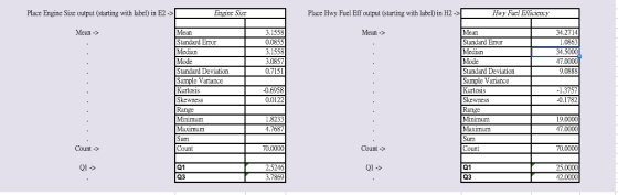
Engine Size
Mean
2.7917
Standard Error
0.0756
Median
2.7917
Mode
2.7297
Standard Deviation
0.6326
Sample Variance
Kurtosis
-0.6958
Skewness
0.0122
Range
Minimum
1.6130
Maximum
4.2186
Sum
Count
70.0000
Q1
2.2954
Q3
3.3191
Hwy Fuel Efficiency
Mean
33.9857
Standard Error
1.0510
Median
35.5000
Mode
46.0000
Standard Deviation
8.7931
Sample Variance
Kurtosis
-1.3320
Skewness
-0.1543
Range
Minimum
19.0000
Maximum
47.0000
Sum
Count
70.0000
Q1
26.0000
Q3
42.0000
The U.S. Department of Energy's Fuel Economy Guide provides fuel...
Just need the answers please.
Engine Size
Mean
2.7917
Standard Error
0.0756
Median
2.7917
Mode
2.7297
Standard Deviation
0.6326
Sample Variance
Kurtosis
-0.6958
Skewness
0.0122
Range
Minimum
1.6130
Maximum
4.2186
Sum
Count
70.0000
Q1
2.2954
Q3
3.3191
Hwy Fuel Efficiency
Mean
33.9857
Standard Error
1.0510
Median
35.5000
Mode
46.0000
Standard Deviation
8.7931
Sample Variance
Kurtosis
-1.3320
Skewness
-0.1543
Range
Minimum
19.0000
Maximum
47.0000
Sum
Count
70.0000
Q1
26.0000
Q3
42.0000
The U.S. Department of Energy's Fuel Economy Guide provides fuel...
I just need help on questions 7 and 8 The U.S. Department of Energy's Fuel Economy...
 I just need help on questions 7 and 8
The U.S. Department of Energy's Fuel Economy Guide provides fuel efficiency data for cars and trucks. (See exercise 35 on page 77 in your textbook for a similar problem.) Use the data in the FuelData sheet in this workbook to generate excel output to answer the following questions. Please note that units are "liters" for engine size and "miles per gallon" for highway fuel efficiency. Put the output in given space...
I just need help on questions 7 and 8
The U.S. Department of Energy's Fuel Economy Guide provides fuel efficiency data for cars and trucks. (See exercise 35 on page 77 in your textbook for a similar problem.) Use the data in the FuelData sheet in this workbook to generate excel output to answer the following questions. Please note that units are "liters" for engine size and "miles per gallon" for highway fuel efficiency. Put the output in given space...
19 ERA 20 Win% 21 0.021 0.028 0.028 0.530 0.038 0.432 0.03 0.022 0.026 0.554 0.028...
 19 ERA 20 Win% 21 0.021 0.028 0.028 0.530 0.038 0.432 0.03 0.022 0.026 0.554 0.028 0.542 0.570 0.620 0.740 0.504 Compute the IQR for ERA. 23 24 25 26 27 28 29 30 31 32 Question 1A Question 1B Compute the covariance between ERA and win%. Question 1C Compute the correlation between ERA and win96. 34 36 Professor Smith took a sample of 211 students from her morning class and a sample of 160 students from her evening class....
Describe one or two general observations you can make about variable X from these results. In...
 Describe one or two general observations you can make about
variable X from these results. In particular, discuss how you would
interpret the Kurtosis and Skewness values based on your reading in
Lane or Devore (or any additional web search you might do on those
topics).
**(IT HAS TO BE BETWEEN 100-200 WORDS)
The results are in the photo
Columnil Mean Standard Error Median Mode Standard Deviation Sample Variance Kurtosis Skewness Range Minimum Maximum Sum Count 97.39902873 2.235602503 95.64542122 11.17801251...
Describe one or two general observations you can make about
variable X from these results. In particular, discuss how you would
interpret the Kurtosis and Skewness values based on your reading in
Lane or Devore (or any additional web search you might do on those
topics).
**(IT HAS TO BE BETWEEN 100-200 WORDS)
The results are in the photo
Columnil Mean Standard Error Median Mode Standard Deviation Sample Variance Kurtosis Skewness Range Minimum Maximum Sum Count 97.39902873 2.235602503 95.64542122 11.17801251...
confused with these questions 3.24. The following data represents the number of days in the hospital...
confused with these questions 3.24. The following data represents the number of days in the hospital for 30 pneumonia patients. 4 4 5 5 5 4 6 5 5 5 2 3 5 3 6 2 4 5 5 7 5 4 3 3 4 5 5 4 4 4 calculate the mean, median, mode, range, variance, standard deviation, Q1,Q3, P60, P20 3.28. Apply the empirical rule to describe the values representing 68 percent, 95 percent, and 99 percent of...
Note: Ahswer Questions S-8 Dy Using the Excel output The U.S. Department of Energy's Fuel Economy...
 Note: Ahswer Questions S-8 Dy Using the Excel output The U.S. Department of Energy's Fuel Economy Guide provides fuel efficiency data for cars and trucks. (See exercise 35 on page 63 in your textbook for a similar problem.) Use the data in the FuelData sheet in this workbook to generate excel output to answer the following questions. Please note that units are "liters" for engine size and "miles per gallon" for highway fuel efficiency. Put the output in given space...
02. 1. Complete the Six Step Process (SSP) as defined Step Process (Version 1)," the Ch....
 02. 1. Complete the Six Step Process (SSP) as defined Step Process (Version 1)," the Ch. 9 & 10 PPT slides and the Wk. 3 SG. You should note that I ha inseited background information and additional notes related to the case within the Excel worksheet in the reference titled"Hypothesis Testing the Six You will need to submit an Excel file containing your statistical output plus a Word document that contains all of your discussion points related to each step...
4. The data below are waiting times (in minutes) for service at a local bank. Also...
 4. The data below are waiting times (in minutes) for service at a local bank. Also included are son summary statistics produced by Excel. Waiting Time Waiting Time Statistics 2.7 3.6 Mean 3.82 1.5 Standard Error 0.61 4.9 Median 3.00 2.8 Mode 2.70 Standard Deviation 2.21 Sample Variance 4.89 Kurtosis 7.79 Skewness 2.55 Range 9.00 Minimum 1.50 Maximum Sum 49.60 Count 13.00 27 4.1 10.50 (Continued) Refer to the bank waiting times data on the previous page. b. Using the...
A study was conducted to evaluate the effectiveness of a weight loss program. Among 36 obese indi...
 A study was conducted to evaluate the effectiveness of a weight loss program. Among 36 obese individuals aged 55 to 75 years randomly selected into the study, each individual had his/her BMI computed before and after the program. The decrease in the BMI was recorded into a SAS dataset and proc univariate was used to analyze this dataset. The population m ean of the decrease in the BMI is denoted by μ. Use the SAS output on the following page...
 Just need the answers please.
Engine Size
Mean
2.7917
Standard Error
0.0756
Median
2.7917
Mode
2.7297
Standard Deviation
0.6326
Sample Variance
Kurtosis
-0.6958
Skewness
0.0122
Range
Minimum
1.6130
Maximum
4.2186
Sum
Count
70.0000
Q1
2.2954
Q3
3.3191
Hwy Fuel Efficiency
Mean
33.9857
Standard Error
1.0510
Median
35.5000
Mode
46.0000
Standard Deviation
8.7931
Sample Variance
Kurtosis
-1.3320
Skewness
-0.1543
Range
Minimum
19.0000
Maximum
47.0000
Sum
Count
70.0000
Q1
26.0000
Q3
42.0000
The U.S. Department of Energy's Fuel Economy Guide provides fuel...
Just need the answers please.
Engine Size
Mean
2.7917
Standard Error
0.0756
Median
2.7917
Mode
2.7297
Standard Deviation
0.6326
Sample Variance
Kurtosis
-0.6958
Skewness
0.0122
Range
Minimum
1.6130
Maximum
4.2186
Sum
Count
70.0000
Q1
2.2954
Q3
3.3191
Hwy Fuel Efficiency
Mean
33.9857
Standard Error
1.0510
Median
35.5000
Mode
46.0000
Standard Deviation
8.7931
Sample Variance
Kurtosis
-1.3320
Skewness
-0.1543
Range
Minimum
19.0000
Maximum
47.0000
Sum
Count
70.0000
Q1
26.0000
Q3
42.0000
The U.S. Department of Energy's Fuel Economy Guide provides fuel...
 I just need help on questions 7 and 8
The U.S. Department of Energy's Fuel Economy Guide provides fuel efficiency data for cars and trucks. (See exercise 35 on page 77 in your textbook for a similar problem.) Use the data in the FuelData sheet in this workbook to generate excel output to answer the following questions. Please note that units are "liters" for engine size and "miles per gallon" for highway fuel efficiency. Put the output in given space...
I just need help on questions 7 and 8
The U.S. Department of Energy's Fuel Economy Guide provides fuel efficiency data for cars and trucks. (See exercise 35 on page 77 in your textbook for a similar problem.) Use the data in the FuelData sheet in this workbook to generate excel output to answer the following questions. Please note that units are "liters" for engine size and "miles per gallon" for highway fuel efficiency. Put the output in given space...
 19 ERA 20 Win% 21 0.021 0.028 0.028 0.530 0.038 0.432 0.03 0.022 0.026 0.554 0.028 0.542 0.570 0.620 0.740 0.504 Compute the IQR for ERA. 23 24 25 26 27 28 29 30 31 32 Question 1A Question 1B Compute the covariance between ERA and win%. Question 1C Compute the correlation between ERA and win96. 34 36 Professor Smith took a sample of 211 students from her morning class and a sample of 160 students from her evening class....
 Describe one or two general observations you can make about
variable X from these results. In particular, discuss how you would
interpret the Kurtosis and Skewness values based on your reading in
Lane or Devore (or any additional web search you might do on those
topics).
**(IT HAS TO BE BETWEEN 100-200 WORDS)
The results are in the photo
Columnil Mean Standard Error Median Mode Standard Deviation Sample Variance Kurtosis Skewness Range Minimum Maximum Sum Count 97.39902873 2.235602503 95.64542122 11.17801251...
Describe one or two general observations you can make about
variable X from these results. In particular, discuss how you would
interpret the Kurtosis and Skewness values based on your reading in
Lane or Devore (or any additional web search you might do on those
topics).
**(IT HAS TO BE BETWEEN 100-200 WORDS)
The results are in the photo
Columnil Mean Standard Error Median Mode Standard Deviation Sample Variance Kurtosis Skewness Range Minimum Maximum Sum Count 97.39902873 2.235602503 95.64542122 11.17801251...
 Note: Ahswer Questions S-8 Dy Using the Excel output The U.S. Department of Energy's Fuel Economy Guide provides fuel efficiency data for cars and trucks. (See exercise 35 on page 63 in your textbook for a similar problem.) Use the data in the FuelData sheet in this workbook to generate excel output to answer the following questions. Please note that units are "liters" for engine size and "miles per gallon" for highway fuel efficiency. Put the output in given space...
 02. 1. Complete the Six Step Process (SSP) as defined Step Process (Version 1)," the Ch. 9 & 10 PPT slides and the Wk. 3 SG. You should note that I ha inseited background information and additional notes related to the case within the Excel worksheet in the reference titled"Hypothesis Testing the Six You will need to submit an Excel file containing your statistical output plus a Word document that contains all of your discussion points related to each step...
 4. The data below are waiting times (in minutes) for service at a local bank. Also included are son summary statistics produced by Excel. Waiting Time Waiting Time Statistics 2.7 3.6 Mean 3.82 1.5 Standard Error 0.61 4.9 Median 3.00 2.8 Mode 2.70 Standard Deviation 2.21 Sample Variance 4.89 Kurtosis 7.79 Skewness 2.55 Range 9.00 Minimum 1.50 Maximum Sum 49.60 Count 13.00 27 4.1 10.50 (Continued) Refer to the bank waiting times data on the previous page. b. Using the...
 A study was conducted to evaluate the effectiveness of a weight loss program. Among 36 obese individuals aged 55 to 75 years randomly selected into the study, each individual had his/her BMI computed before and after the program. The decrease in the BMI was recorded into a SAS dataset and proc univariate was used to analyze this dataset. The population m ean of the decrease in the BMI is denoted by μ. Use the SAS output on the following page...
Most questions answered within 3 hours.
-
Where is the error in this code sequence?
String s1 = "Hello";
String s2 = "ello";...
asked 10 months ago -
Financial data for Joel de Paris, Inc., for last year
follow:
Joel de Paris, Inc.
Balance...
asked 10 months ago -
Consider this reaction:
Al2(SO4)3 (aq)+ BaCl3
(aq) Al2Cl6 (aq)- +
3BaSO4(s) . What is the...
asked 10 months ago -
Suppose that Savneet is considering increasing her
recent random sample from 20 car rentals to 40...
asked 10 months ago -
Trucks arrive at an unloading terminal at an average rate of 120
per hour.
Trucks arrive...
asked 10 months ago -
Why are methanol and ethanol completely soluble in water while
octanol is not very little soluble....
asked 10 months ago -
A facilities manager at a university reads in a research report
that the mean amount of...
asked 10 months ago -
When the CuSO4 is rehydrated by adding water to the anhydrous
compound, is this an endothermic...
asked 10 months ago -
A ray of sunlight is passing from diamond into crown glass; the
angle of incidence is...
asked 10 months ago -
A block of mass 0.249 kg is placed on top of a light, vertical
spring of...
asked 10 months ago -
how do the kidneys compensate in the presences of acidosis
a) trigger hyperventilate
b) reserve acid...
asked 10 months ago -
Question 501 pts
The rental rate of capital to the firm increases. Which of the
following...
asked 10 months ago