Question

Please answer this question with RStudio.

4. In this problem, you will illustrate the idea of resampling and sampling distributions. A ganma distribution with shape k and scale θ has density exp(-v/0) Assume shape k = 2 and scale θ = 3 (a) Use the function dgamma in R to evaluate the density for a range of values between 0 and 20. Produce a plot of the density (b) The (true) mean and variance of the gamma distribution are simple functions of the shape and scale parameters. Use the internet (Wikipedia is fine) to find the true mean μ, variance σ2, and standard deviation σ of the distribution described in (a) (c) Assume we take a sample of size n- 12 where X, are iid random variables with gamma distributions with shape k = 2 and scale θ = 3 and we calculate X = 1/12 ΣΙ, x, . 1s X random? Explain (d) Give the true mean ,48, variance σ, and standard deviation ơX, of X in (c) Test statistics are usually standardized so that standard tables can be used. The distribution of interest is the distribution of X. To standardize, one subtracts off the mean, and divides by the standard deviation. The trick is, usually the true mean and true standard deviation aren't known. It turns out that in a test for means, the fact that the true mean is unknown is not a problem because we hypothesize the true mean with the null hypothesis. However, the fact that the standard deviation is unknown does make a difference, as we illustrate below. (e) Use rgamma to generate a sample of sizen 12 from a gamma distribution with shape k-2 and scale θ-3. Calculate the sample mean m. Suppose our null hypothesis is Ho : μ-6. Calculate the test statistic Z-ms- m .. Note: This test statistic assumes the true standard deviation is known. Use a for-loop to repeatedly calculate the test statistic and store these values. Plot a histogram of the test statistics, and use dnorm to overlay a standard normal density. You may want to adjust the histogram settings, look at the help page: ?hist, and you will want to set freqF to compare with the normal density. Does the distribution of this test statistic appear to be well approximated by a standard normal? (f) Repeat (e), but now using the test statistic T = -2, where 8 is the sample standard deviation. Does the distribution of this test statistic appear to be well approximated by a standard normal? Use R to draw the density curve of a more appropriate distribution

Answer 1

R code with comments (all statements starting with # are comments)

#set the parameters of gamma distribution
k<-2
theta<-3
#part a)
#set the values of x
x<-seq(0,20,length=100)
#get the density of x
p<-dgamma(x,shape=k,scale=theta)
#plot
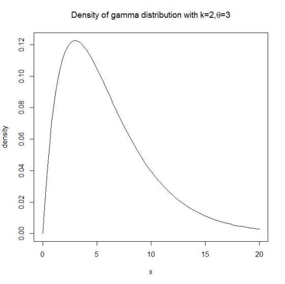
plot(x,p,type="l",ylab="density",main=bquote("Density of gamma distribution with k=2,"*theta*"=3"))

#get this plot

b) The expected value (true mean) of X is

$\mu=E(X)=k\theta=2\times 3=6$

the variance of X is

$\sigma^2=Var(X)=k\theta^2=2\times 3^2=18$

#part b)
#expected value is
mu<-k*theta
sigma2<-k*theta^2
sprintf('The true mean of X is %.4f',mu)
sprintf('The true variance of X is %.4f',sigma2)

#get this poutput

c) Each sample of size 12 is a draw from Gamma distribution and they are different.

Since $X_i$s are random variables, the sum

$\sum_{i=1}^{12}X_i$ is also a random variable.

If we divide this sum by n, the average that we get of these $X_i$s is also random.

Hence $\bar{X}=\frac{\sum_{i=1}^{12}X_i}{12}$ is a random variable.

d) the true mean of $\bar{X}$ is

$\mu_{\bar{X}}=\mu=6$

The true variance of $\bar{X}$ is

$\sigma^2_{\bar{X}}=\frac{\sigma^2}{n}=\frac{18}{12}=1.5$

The true standard deviation of $\bar{X}$ is

$\sigma_{\bar{X}}=\sqrt{\sigma^2_{\bar{X}}}=\sqrt{1.5}=1.225$

R code

#part d)
#set the sample size
n<-12
#get the true mean of sample mean
muxbar<-mu
#get the true variance of sample mean
sigma2xbar<-sigma2/n
#get the true standard deviation of sample mean
sigmaxbar<-sqrt(sigma2xbar)

sprintf('The true mean of sample mean is %.4f',muxbar)
sprintf('The true variance of sample mean is %.4f',sigma2xbar)
sprintf('The true standard deviation of sample mean is %.4f',sigmaxbar)

#get this output

e) R code

#part e)
#set the random seed
set.seed(123)
#set the sample size
n<-12
#set the number of repetition
r<-10000
#intialize the variable to store the z values
z<-numeric(r)
for (i in 1:r) {
    x<-rgamma(n,shape=k,scale=theta)
   #get the sample mean m
   m<-mean(x)
   #calculate the test statistics
   z[i]<-(m-6)/sigmaxbar
}
#plot the histogram of z
hist(z,breaks=50,freq=FALSE,xlab="Test statistics (z)",main="Histogram of the test statistics")
#add dnorm
curve(dnorm(x),from=min(z),to=max(z),add=TRUE,col="red")

#get this plot

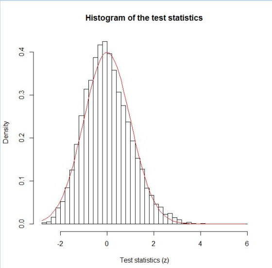
The distribution of the test statistics is reasonably well approximated by a normal distribution.

f) Using sample standard deviation

#part f)
#set the random seed
set.seed(123)
#set the sample size
n<-12
#set the number of repeatition
r<-10000
#intialize the variable to store the z values
t<-numeric(r)
for (i in 1:r) {
    x<-rgamma(n,shape=k,scale=theta)
   #get the sample mean m
   m<-mean(x)
   #get the sample standard deviation
   s<-sd(x)
   #calculate the test statistics
   t[i]<-(m-6)/(s/sqrt(n))
}
#plot the histogram of t
hist(t,breaks=50,freq=FALSE,xlab="Test statistics (t)",main="Histogram of the test statistics",ylim=c(0,0.4))
#add dnorm
curve(dnorm(x),from=min(t),to=max(t),add=TRUE,col="red")
#add dt
curve(dt(x,df=n-1),from=min(t),to=max(t),add=TRUE,col="blue")
legend("topleft",c("test statistics","standard normal","standard t"),lty=1,col=c("black","red","blue"))

#get this plot

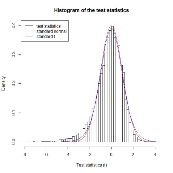
t distribution with its thicket tail seems to be a better fit than standard normal, particularly for the left tail.