Question

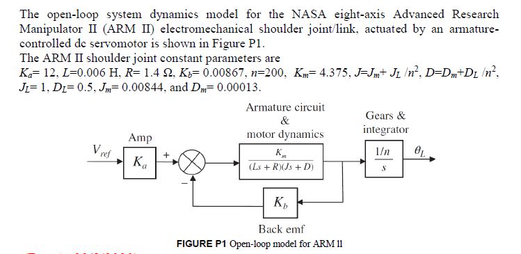
The open-loop system dynamics model for the NASA eight-axis Advanced Research Manipulator II (ARM II) electromechanical shoulder joint/link, actuated by an armature-controlled dc servomotor is shown in Figure P1.

The ARM II shoulder joint constant parameters are

Ka= 12, L=0.006 H, R= 1.4 Ω, Kb= 0.00867, n=200, Km= 4.375, J=Jm+ JL /n2, D=Dm+DL /n2, JL= 1, DL= 0.5, Jm= 0.00844, and Dm= 0.00013.

FIGURE P1 Open-loop model for ARM ll

(Due to 29/8/2020)

a. Obtain the equivalent open-loop transfer function, ?(?) (with a unity feedback system) (using MatLab or MatLab/Simulink).

b. The loop is to be closed by cascading a controller, Gc1(s) = KP, with G(s) in the forward path forming an equivalent forward-transfer function, Ge(s) = Gc1(s) G(s). Parameters of Gc1(s) will be used to design a desired transient performance. The input to the closed-loop system is a voltage, VI(s), representing the desired angular displacement of the robotic joint with a ratio of 1 volt equals 1 radian. The output of the closed-loop system is the actual angular displacement of the joint, θL(s). An encoder in the feedback path, Ke, converts the actual joint displacement to a voltage with a ratio of 1 radian equals 1 volt. Draw the closed loop system showing all transfer functions. (Use Microsoft PowerPoint or Visio to draw the system)

c. Find the closed-loop transfer function ?(?). (using MatLab or MatLab/Simulink).

d. Determine the range of KP for which the system is stable (using root locus technique).

e. Determine the step response for four different values of KP including stability and instability conditions (using MatLab or MatLab/Simulink).

f. Determine the transient parameters for a selected stable oscillatory response (rising time, settling time, overshoot (if exists) and compare and discuss the response (using MatLab or MatLab/Simulink). (choose a value for KP)

g. What is the min. steady state error of this system?

Capture.JPG