Question

question #1 A-D. Please show work.

Q1. The following Regression function has been developed to check the relationship between the dependent variable y and the independent variable x1. Consider the following Minitab output and answer the questions. Regression Equation 9 = 0.86 + 0.65 x1 a) (4pt). Please fill out the Coefficients table appropriately. Coefficients Term Coef SE Coef T-Value P-Value VIF Constant (1) 1.38 16.58 0.000 X1 (ii) 0.231 7.00 0.000 1.00

Answer 1

a)

i) Coefficient for Constant = 1.38*16.58 = 22.8804

ii) Coefficient for x1 = 0.231*7 = 1.617

---

b)

iii) df(Regression) = 1

iv) df(error) = 9-1 = 8

v) SSE = 3.10 - 2.12 = 0.98

---

c)

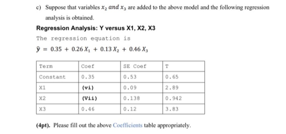
vi) Coefficient for x1 = 0.09*2.89 = 0.26

vii) Coefficient for x2 = 0.138*0.942 = 0.13

---

d)

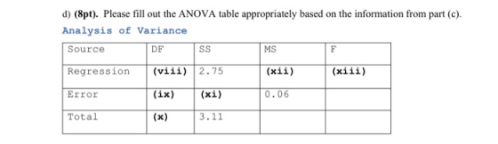
viii) df(Regression) = 3

xi) SSE = 3.11 - 2.75 = 0.36

ix) df(error) = .36/.06 = 6

x) df(total) = 3+6 = 9

xii) MSR = 2.75/3 = 0.9167

xiii) F = MSR/MSE = .9167/.06 = 15.2778

ANOVA
	df	SS	MS	F
Regression	3	2.75	0.9167	15.2778
Residual	6	0.36	0.06
Total	9	3.11