Question

A small Internet company wants to determine how the money they spend on Google Adwords impacts their monthly revenue. Over 6 consecutive months, they vary the amount they spend on their Adwords campaign in $) and record the associated revenue (in %) for each month. The data is shown below. Assignment 1092 data a) Develop a regression equation for predicting monthly revenue based on the amount spent with Adwords. What is the y- intercept? Give your answer to two decimal places. b) What is the proper interpretation of the y-intercept in the regression equations? The y-intercept describes the expected increase in revenue for each additional dollar spent on Adwords. The y-intercept describes the expected decrease in revenue for each additional dollar spent on Adwords. The y-intercept describes the expected revenue if the company spends $25 in a given month on Adwords. The y-intercept describes the expected revenue if the company does not spend any money in a given month on Adwords. c) What is the sample correlation between these two variables? Give your answer to two decimal places. d) What is the slope of your regression equation? Give your answer to two decimal places. e) Using a 0.05 level of significance, does this regression equation appear to have any value for predicting revenue based on Adwords expenditures? No because there is a significant linear relationship between the two quantities. Yes because there is not a significant linear relationship between the two quantities. Yes because there is a significant linear relationship between the two quantities. No because there is not a significant linear relationship between the two quantities.

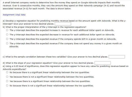
Adwords	Revenue
50	427
75	472
100	467
125	529
150	518
175	543

Answer 1

I have attached the complete R code below as well as the output

> x=c(50,75,100,125,150,175)
> y=c(427,472,467,529,518,543)
> model=lm(y~x);model

Call:
lm(formula = y ~ x)

Coefficients:
(Intercept)            x  
   392.3810       0.8914  

> summary(model)

Call:
lm(formula = y ~ x)

Residuals:
      1       2       3       4       5       6 
 -9.952  12.762 -14.524  25.190  -8.095  -5.381 

Coefficients:
            Estimate Std. Error t value Pr(>|t|)    
(Intercept) 392.3810    19.9443  19.674 3.94e-05 ***
x             0.8914     0.1657   5.378  0.00578 ** 
---
Signif. codes:  0 ‘***’ 0.001 ‘**’ 0.01 ‘*’ 0.05 ‘.’ 0.1 ‘ ’ 1

Residual standard error: 17.33 on 4 degrees of freedom
Multiple R-squared:  0.8785,    Adjusted R-squared:  0.8481 
F-statistic: 28.93 on 1 and 4 DF,  p-value: 0.005775

> cor(x,y)
[1] 0.9372906

a) 392.38

As it can be observed from the output that the intercept is 392.38

b) Option D

The regression line is given by

y=392.38+0.8914*x

So when x that is Adwords is equal to 0 then the expected revenue is 392.38.

Hence option D is correct

c) 0.94

It can be seen from the output that the sample correlation is equal to 0.94 after rounding up which implies that both x and y are highly correlated with each other that is when one increases both also increases.

d) 0.89

The slope of the regression line after rounding up is 0.89 which implies that for a unit increase in Adwords the expected revenue increases by a 0.89.

e) Option C

As seen in the output the p-value for the final regression line is 0.005775 which is smaller than 0.05 which implies that the regression line is significant.

As the regression line is significant we can use the line for prediction purpose.

Do comment if you have any doubt.

Thank you !!