Question

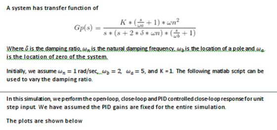
It has the following transfer function:

$Gp(s)=\frac{K*(\frac{s}{\omega a}+1)*\omega n^2}{s*(s+2* \delta * \omega n)*(\frac{s}{ \omega b}+1)}$

-What happens to the plant with different values of ($\delta$) (relative damping factor), also analyze how it influences if the values of $\omega n$ , $\omega a$   and $\omega b$ vary, for this implement scripts in Matlab.m and show the results in graphs
corresponding.
- Implement models of transfer functions in:
a) open loop
b) closed loop with unit feedback
b) closed loop with unit feedback and a PID controller

-what are the values of $\omega n$ , $\omega a$   and $\omega b$ called

Answer 1

A system has transfer function of Gp(s) K* ( + 1) *wn? S*(s + 2* S*wn) * (+1) Where is the damping.catie Wn is the natural damping frequency. W is the location of a pole and be is the location of zero of the system Initially, we assume wn = 1 rad/secW; = 2, wa = 5, and K = 1. The following matlab script can be used to vary the damping ratio. In this simulation, we perform the open-loop, close-loop and PID controlled close loop response for unit step input We have assumed the PID gains are fixed for the entire simulation. The plots are shown below

clear all
clc
s = tf('s');
%% model the system
wn = 1; % in rad/sec
wb = 2;
wa = 5;
K = 1;
% Varying the parameter zeta
zeta = [0;0.2;0.4;0.8;1];
% time of simulation
time = 0:0.1:10;
% control input
u = ones(1,length(time));

for i = 1:length(zeta)
  
    % model the transfer function
    Gp = (K*(s/wa + 1)*wn^2)/(s*(s + 2*zeta(i)*wn)*(s/wb + 1));
  
    % compute the open-loop TF for step input
    [y,t] = lsim(Gp,u,time);
    y_ol(:,i) = y;
  
    % model the close-loop TF with unity feedback
    Tp = feedback(Gp,1);
  
    % compute the close-loop TF for step input
    [y_c,t_c] = lsim(Tp,u,time);
    y_cl(:,i) = y_c;
  
    % PID controller TF
    Kp = 10;
    Ki = 1;
    Kd = 0.1;
    Gc = pid(Kp,Ki,Kd);
  
    % model the close-loop TF with PID controller
    Tpid = feedback(Gp*Gc,1);
  
    % compute the PID controlled close-loop TF for step input
    [y_p,t_p] = lsim(Tpid,u,time);
    y_pid(:,i) = y_p;
  
end

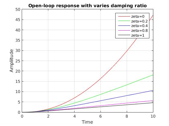
% plot the open-loop response
figure(1)
plot(time,y_ol(:,1),'r')
hold on
plot(time,y_ol(:,2),'g')
hold on
plot(time,y_ol(:,3),'b')
hold on
plot(time,y_ol(:,4),'m')
hold on
plot(time,y_ol(:,5),'k')
grid
xlabel('Time')
ylabel('Amplitude')
legend('zeta=0','zeta=0.2','zeta=0.4','zeta=0.8','zeta=1')
title('Open-loop response with varies damping ratio')

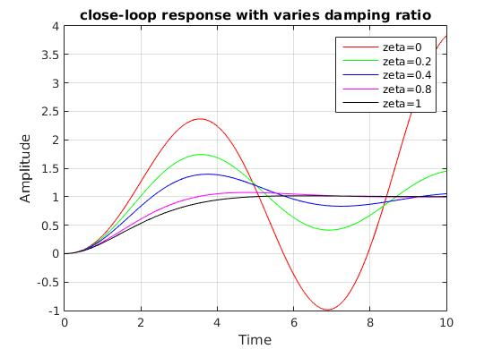
% plot the close-loop response
figure(2)
plot(time,y_cl(:,1),'r')
hold on
plot(time,y_cl(:,2),'g')
hold on
plot(time,y_cl(:,3),'b')
hold on
plot(time,y_cl(:,4),'m')
hold on
plot(time,y_cl(:,5),'k')
grid
xlabel('Time')
ylabel('Amplitude')
legend('zeta=0','zeta=0.2','zeta=0.4','zeta=0.8','zeta=1')
title('close-loop response with varies damping ratio')

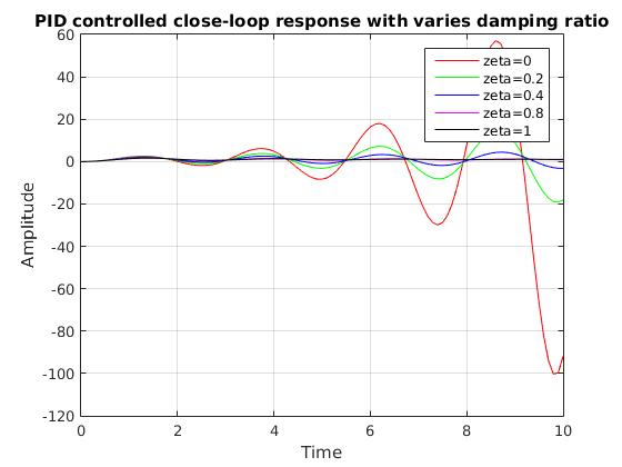
% plot the PID controlled close-loop response
figure(3)
plot(time,y_pid(:,1),'r')
hold on
plot(time,y_pid(:,2),'g')
hold on
plot(time,y_pid(:,3),'b')
hold on
plot(time,y_pid(:,4),'m')
hold on
plot(time,y_pid(:,5),'k')
grid
xlabel('Time')
ylabel('Amplitude')
legend('zeta=0','zeta=0.2','zeta=0.4','zeta=0.8','zeta=1')
title('PID controlled close-loop response with varies damping ratio')

Open-loop response with varies damping ratio 50 45 zeta=0 zeta=0.2 zeta=0.4 zeta=0.8 zeta=1 40 35 30 Amplitude 25 20 15 10 5 0 4 09 8 10 IN Time

close-loop response with varies damping ratio 4 3. 5 zeta=0 zeta=0.2 zeta=0.4 zeta=0.8 zeta=1 3 2 5 2 Amplitude 1.5 1 0.5 0 -0.5 -1 0 2 4 LO 8 10 Time

PID controlled close-loop response with varies damping ratio 40 zeta=0 zeta=0.2 zeta=0.4 zeta=0.8 zeta=1 20 0 -20 Amplitude -40 -60 -80 -100 -120 2 4 6 8 10 Time

Now, we are varying the parameter W, while assume , 0 = 1, w; = 2, wa = 5, and K = 1 The correspondingmatlab script for the same is shown below. In this simulation, we perform the open-loop, close-loop and PID controlled close-loop response for unit step input We have assumed the PID gains are fixed for the entire simulation.

clear all
clc
s = tf('s');
%% model the system
zeta = 1; % damping ratio
wb = 2;
wa = 5;
K = 1;
% Varying the parameter wn
wn = [0;2;4;8;10];
% time of simulation
time = 0:0.1:10;
% control input
u = ones(1,length(time));

for i = 1:length(wn)
  
    % model the trnasfer function
    Gp = (K*(s/wa + 1)*wn(i)^2)/(s*(s + 2*zeta*wn(i))*(s/wb + 1));
  
    % compute the open-loop TF for step input
    [y,t] = lsim(Gp,u,time);
    y_ol(:,i) = y;
  
    % model the close-loop TF with unity feedback
    Tp = feedback(Gp,1);
  
    % compute the close-loop TF for step input
    [y_c,t_c] = lsim(Tp,u,time);
    y_cl(:,i) = y_c;
  
    % PID controller TF
    Kp = 10;
    Ki = 1;
    Kd = 0.1;
    Gc = pid(Kp,Ki,Kd);
  
    % model the close-loop TF with PID controller
    Tpid = feedback(Gp*Gc,1);
  
    % compute the PID controlled close-loop TF for step input
    [y_p,t_p] = lsim(Tpid,u,time);
    y_pid(:,i) = y_p;
  
end

% plot the open-loop response
figure(1)
plot(time,y_ol(:,1),'r')
hold on
plot(time,y_ol(:,2),'g')
hold on
plot(time,y_ol(:,3),'b')
hold on
plot(time,y_ol(:,4),'m')
hold on
plot(time,y_ol(:,5),'k')
grid
xlabel('Time')
ylabel('Amplitude')
legend('wn=0','wn=2','wn=4','wn=8','wn=10')
title('Open-loop response with varies wn')

% plot the close-loop response
figure(2)
plot(time,y_cl(:,1),'r')
hold on
plot(time,y_cl(:,2),'g')
hold on
plot(time,y_cl(:,3),'b')
hold on
plot(time,y_cl(:,4),'m')
hold on
plot(time,y_cl(:,5),'k')
grid
xlabel('Time')
ylabel('Amplitude')
legend('wn=0','wn=2','wn=4','wn=8','wn=10')
title('close-loop response with varies wn')

% plot the PID controlled close-loop response
figure(3)
plot(time,y_pid(:,1),'r')
hold on
plot(time,y_pid(:,2),'g')
hold on
plot(time,y_pid(:,3),'b')
hold on
plot(time,y_pid(:,4),'m')
hold on
plot(time,y_pid(:,5),'k')
grid
xlabel('Time')
ylabel('Amplitude')
legend('wn=0','wn=2','wn=4','wn=8','wn=10')
title('PID controlled close-loop response with varies wn')

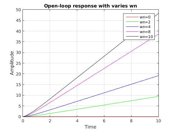
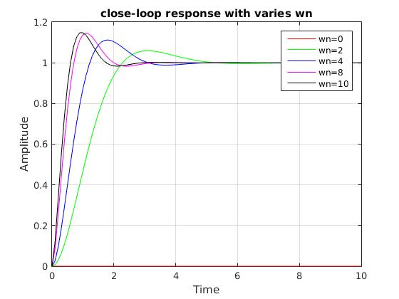
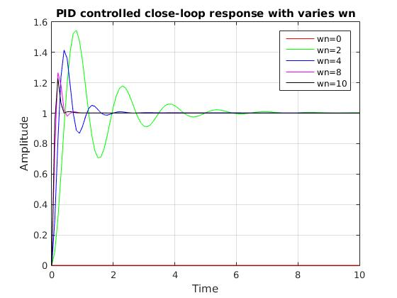
The corresponding plots are shown below

Open-loop response with varies wn 50 45 wn=0 wn=2 wn=4 wn=8 wn=10 40 35 30 Amplitude 25 20 15 10 5 0 4 6 8 10 N Time

close-loop response with varies wn 1.2 1 wn=0 wn=2 wn=4 wn=8 wn=10 0.8 Amplitude 0.6 0.4 0.2 0 4 6 8 10 N Time

PID controlled close-loop response with varies wn 1.6 1.4 wn=0 wn=2 wn=4 wn=8 wn=10 1.2 Amplitude 0.8 0.6 0.4 0.2 0 2 4 6 8 10 Time

Now, we are varying the parameter.wa, while assume , ô = 1, n = 10 rad/sec, wa = 5, and K=1. The corresponding matlab script for the same is shown below. In this simulation, we perform the open- loop, close-loop and PID controlled close-loop response for unit step input We have assumed the PID gains are fixed for the entire simulation.

clear all
clc
s = tf('s');
%% model the system
zeta = 1; % damping ratio
wn = 10; % rad/sec
wa = 5;
K = 1;
% Varying the parameter wb
wb = [1;2;4;8;10];
% time of simulation
time = 0:0.1:10;
% control input
u = ones(1,length(time));

for i = 1:length(wb)
  
    % model the trnasfer function
    Gp = (K*(s/wa + 1)*wn^2)/(s*(s + 2*zeta*wn)*(s/wb(i) + 1));
  
    % compute the open-loop TF for step input
    [y,t] = lsim(Gp,u,time);
    y_ol(:,i) = y;
  
    % model the close-loop TF with unity feedback
    Tp = feedback(Gp,1);
  
    % compute the close-loop TF for step input
    [y_c,t_c] = lsim(Tp,u,time);
    y_cl(:,i) = y_c;
  
    % PID controller TF
    Kp = 10;
    Ki = 1;
    Kd = 0.1;
    Gc = pid(Kp,Ki,Kd);
  
    % model the close-loop TF with PID controller
    Tpid = feedback(Gp*Gc,1);
  
    % compute the PID controlled close-loop TF for step input
    [y_p,t_p] = lsim(Tpid,u,time);
    y_pid(:,i) = y_p;
  
end

% plot the open-loop response
figure(1)
plot(time,y_ol(:,1),'r')
hold on
plot(time,y_ol(:,2),'g')
hold on
plot(time,y_ol(:,3),'b')
hold on
plot(time,y_ol(:,4),'m')
hold on
plot(time,y_ol(:,5),'k')
grid
xlabel('Time')
ylabel('Amplitude')
legend('wb=1','wb=2','wb=4','wb=8','wb=10')
title('Open-loop response with varies wb')

% plot the close-loop response
figure(2)
plot(time,y_cl(:,1),'r')
hold on
plot(time,y_cl(:,2),'g')
hold on
plot(time,y_cl(:,3),'b')
hold on
plot(time,y_cl(:,4),'m')
hold on
plot(time,y_cl(:,5),'k')
grid
xlabel('Time')
ylabel('Amplitude')
legend('wb=1','wb=2','wb=4','wb=8','wb=10')
title('close-loop response with varies wb')

% plot the PID controlled close-loop response
figure(3)
plot(time,y_pid(:,1),'r')
hold on
plot(time,y_pid(:,2),'g')
hold on
plot(time,y_pid(:,3),'b')
hold on
plot(time,y_pid(:,4),'m')
hold on
plot(time,y_pid(:,5),'k')
grid
xlabel('Time')
ylabel('Amplitude')
legend('wb=1','wb=2','wb=4','wb=8','wb=10')
title('PID controlled close-loop response with varies wb')

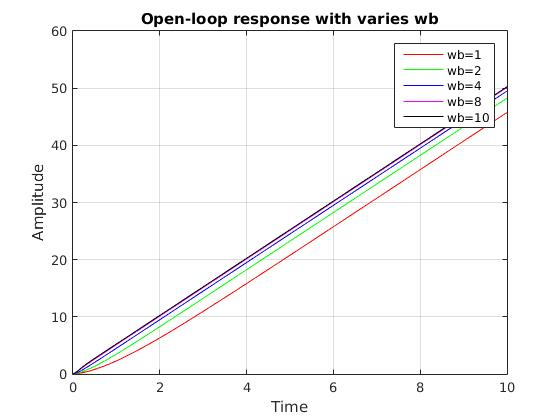
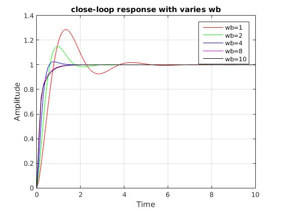
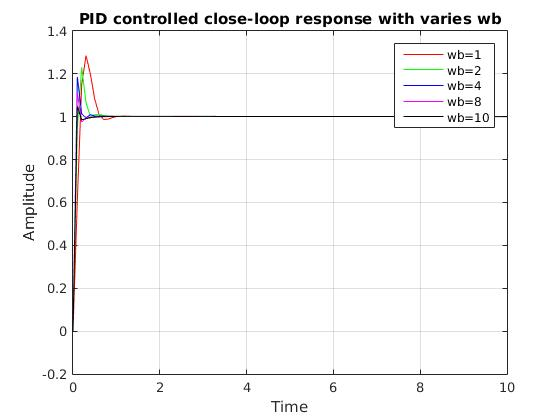
The corresponding responses are shown below

Open-loop response with varies wb 60 50 wb=1 wb=2 wb=4 wb=8 wb=10 40 Amplitude 30 20 10 4 6 8 10 N Time

close-loop response with varies wb 1.4 1.2 wb=1 wb=2 wb=4 wb=8 wb=10 1 0.8 Amplitude 0.6 0.4 0.2 2 4 6 8 10 Time

PID controlled close-loop response with varies wb 1.4 1.2 wb=1 wb=2 wb=4 wb=8 wb=10 1 0.8 Amplitude 0.6 1.4 0.2 0 -0.2 4 6 8 10 IN Time

Now, we are varying the parameter.wa, while assume, ô = 1, Wn= 10 rad/sec, W; = 10, and K=1. The corresponding matlab script for the same is shown below. In this simulation, we perform the open- loop, close-loop and PID controlled close-loop response for unit step input Wehave assumed the PID gains are fixed for the entire simulation.

clear all
clc
s = tf('s');
%% model the system
zeta = 1; % damping ratio
wn = 10; % rad/sec
wb = 5;
K = 1;
% Varying the parameter wb
wa = [2;4;6;8;10];
% time of simulation
time = 0:0.1:10;
% control input
u = ones(1,length(time));

for i = 1:length(wa)
  
    % model the trnasfer function
    Gp = (K*(s/wa(i) + 1)*wn^2)/(s*(s + 2*zeta*wn)*(s/wb + 1));
  
    % compute the open-loop TF for step input
    [y,t] = lsim(Gp,u,time);
    y_ol(:,i) = y;
  
    % model the close-loop TF with unity feedback
    Tp = feedback(Gp,1);
  
    % compute the close-loop TF for step input
    [y_c,t_c] = lsim(Tp,u,time);
    y_cl(:,i) = y_c;
  
    % PID controller TF
    Kp = 10;
    Ki = 1;
    Kd = 0.1;
    Gc = pid(Kp,Ki,Kd);
  
    % model the close-loop TF with PID controller
    Tpid = feedback(Gp*Gc,1);
  
    % compute the PID controlled close-loop TF for step input
    [y_p,t_p] = lsim(Tpid,u,time);
    y_pid(:,i) = y_p;
  
end

% plot the open-loop response
figure(1)
plot(time,y_ol(:,1),'r')
hold on
plot(time,y_ol(:,2),'g')
hold on
plot(time,y_ol(:,3),'b')
hold on
plot(time,y_ol(:,4),'m')
hold on
plot(time,y_ol(:,5),'k')
grid
xlabel('Time')
ylabel('Amplitude')
legend('wa=2','wa=4','wa=6','wa=8','wa=10')
title('Open-loop response with varies wa')

% plot the close-loop response
figure(2)
plot(time,y_cl(:,1),'r')
hold on
plot(time,y_cl(:,2),'g')
hold on
plot(time,y_cl(:,3),'b')
hold on
plot(time,y_cl(:,4),'m')
hold on
plot(time,y_cl(:,5),'k')
grid
xlabel('Time')
ylabel('Amplitude')
legend('wa=2','wa=4','wa=6','wa=8','wa=10')
title('close-loop response with varies wa')

% plot the PID controlled close-loop response
figure(3)
plot(time,y_pid(:,1),'r')
hold on
plot(time,y_pid(:,2),'g')
hold on
plot(time,y_pid(:,3),'b')
hold on
plot(time,y_pid(:,4),'m')
hold on
plot(time,y_pid(:,5),'k')
grid
xlabel('Time')
ylabel('Amplitude')
legend('wa=2','wa=4','wa=6','wa=8','wa=10')
title('PID controlled close-loop response with varies wa')

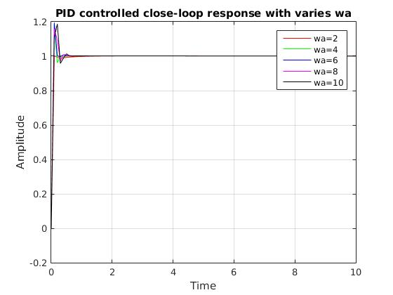
The corresponding responses are shown below

Open-loop response with varies wa 60 50 wa=2 wa=4 wa=6 wa=8 wa=10 40 Amplitude 30 20 10 o 4 6 8 10 IN Time

close-loop response with varies wa 1 2 1 wa=2 wa=4 wa=6 wa=8 wa=10 0.8 Amplitude 0.6 0.4 0.2 0 4 6 8 10 IN Time

PID controlled close-loop response with varies wa 1 1.2 1 wa=2 wa=4 wa=6 wa=8 wa=10 0.8 0.6 Amplitude 1.4 0.2 0 -0.2 4 6 8 10 IN Time

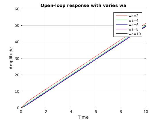
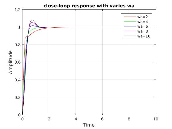
Here, Where δ is the damping ratio, ω_n is the natural damping frequency, ω_b is the location of a pole and ω_a is the location of zero of the system.