
Homework Answers

Add Answer to:
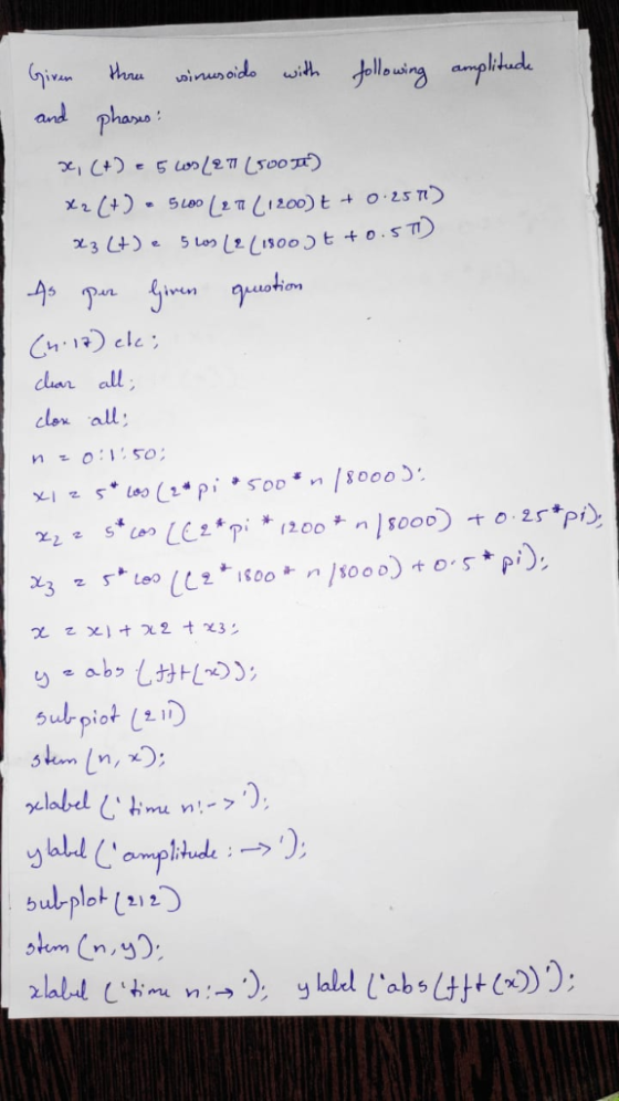
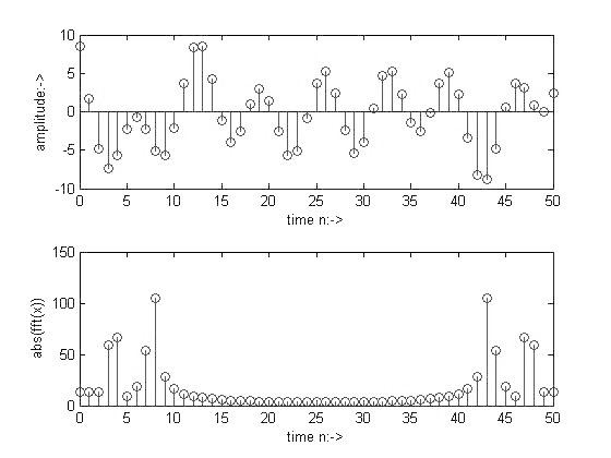
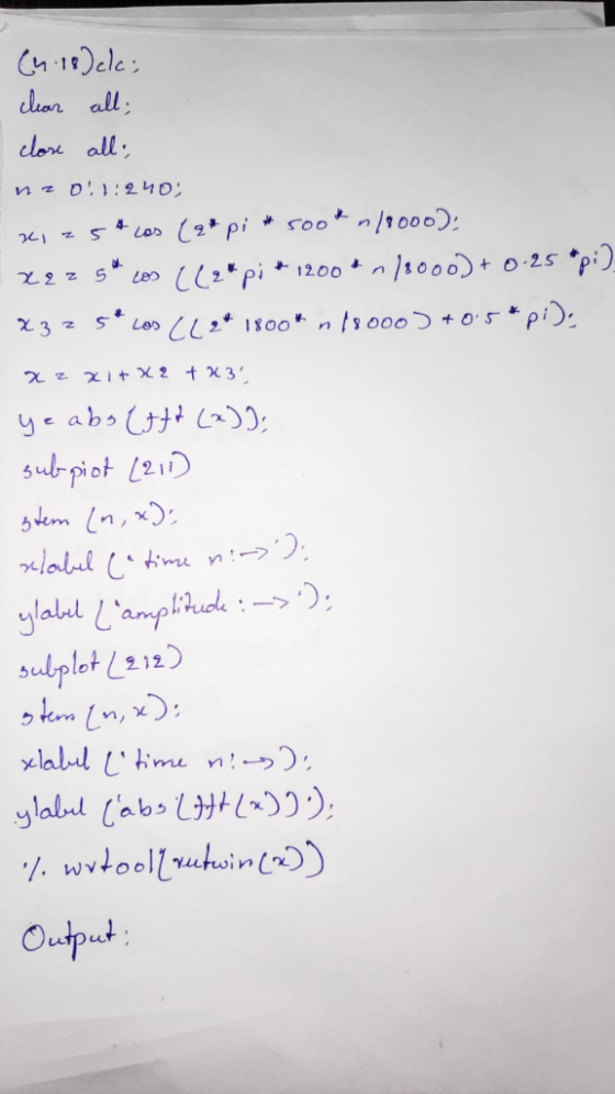
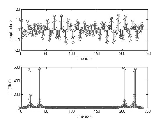
3) Given three sinusoids with the following amplitude and phases (t)-Scos(2x (1200+0.25x) a. Create a MATLAB...
3) Given three sinusoids with the following amplitude and phases (t)-Scos(2x (1200+0.25x) a. Crea...
 3) Given three sinusoids with the following amplitude and phases (t)-Scos(2x (1200+0.25x) a. Create a MATLAB program to sample each sinusoid and generate a sum of three sinusoids, that is, х(n)=x1(nHx:(n)+xy(n), using a sampling rate of 8000 Hz, and plot the sum x(n) over a range of time that will exhibit approximately 0.1 second. (10 pts) b. Use the MATLAB function fO to compute DFT coefficients, and plot and examine the spectrum of the signal x(n).(10 pts Write a MATLAB...
MATLAB Code Question alpha = 2.3 beta = 4.3 zeta = 9.1 PROBLEM 4 (20 points). Consider three sinusoids with the following amplitudes and phases a.cs(2n(500t)) β.cos(2n(500t) +0.5r) x1n] x2[n] rn...
 MATLAB Code Question
alpha = 2.3
beta = 4.3
zeta = 9.1
PROBLEM 4 (20 points). Consider three sinusoids with the following amplitudes and phases a.cs(2n(500t)) β.cos(2n(500t) +0.5r) x1n] x2[n] rn = cos(2(500t)0.75) Create a MATLAB program to sample each sinusoid and generate a sum of three sinusoids, that is using a sampling rate of 8,000 Hz over a range of 0.1 seconds Use the MATLAB function stem) to plot r[n] for the first 20 samples Use the MATLAB function...
MATLAB Code Question
alpha = 2.3
beta = 4.3
zeta = 9.1
PROBLEM 4 (20 points). Consider three sinusoids with the following amplitudes and phases a.cs(2n(500t)) β.cos(2n(500t) +0.5r) x1n] x2[n] rn = cos(2(500t)0.75) Create a MATLAB program to sample each sinusoid and generate a sum of three sinusoids, that is using a sampling rate of 8,000 Hz over a range of 0.1 seconds Use the MATLAB function stem) to plot r[n] for the first 20 samples Use the MATLAB function...
Need MatLab code Exercise: Use MATLAB to generate the sinusoidal waveform: x(t) = 3 cos(1200) Consider...
 Need MatLab code
Exercise: Use MATLAB to generate the sinusoidal waveform: x(t) = 3 cos(1200) Consider the frequency of this sinusoid and use this information to select an appropriate time-step and time array that will allow this signal to be correctly represented and displayed on a new MATLAB figure window (display 4 periods of this wave only). Now set up an appropriate frequency array and use the fft() and fftshift() functions to generate and plot the Fourier Transform (magnitude spectra)...
Need MatLab code
Exercise: Use MATLAB to generate the sinusoidal waveform: x(t) = 3 cos(1200) Consider the frequency of this sinusoid and use this information to select an appropriate time-step and time array that will allow this signal to be correctly represented and displayed on a new MATLAB figure window (display 4 periods of this wave only). Now set up an appropriate frequency array and use the fft() and fftshift() functions to generate and plot the Fourier Transform (magnitude spectra)...
(B) Implement Matlab code for each part as described below: i) Define the following signal in tim...
 Using MATLAB, Please read carefully, EXPLAIN CODE AND ANSWERS,
DISCUSS RESULTS, I NEED EVERY PART
(B) Implement Matlab code for each part as described below: i) Define the following signal in time and plot it where Ai 10, A2-3, fi-10 Hz, f2-40 Hz. part of the DFT, and discuss the results. zero. Do this carefully for both positive and negative frequencies. Call this signal G (f). ii) Compute the DFT S(f) of s (t) using the fft() function. Plot the...
Using MATLAB, Please read carefully, EXPLAIN CODE AND ANSWERS,
DISCUSS RESULTS, I NEED EVERY PART
(B) Implement Matlab code for each part as described below: i) Define the following signal in time and plot it where Ai 10, A2-3, fi-10 Hz, f2-40 Hz. part of the DFT, and discuss the results. zero. Do this carefully for both positive and negative frequencies. Call this signal G (f). ii) Compute the DFT S(f) of s (t) using the fft() function. Plot the...
Please can you solve it using MATLAB. (1) Generate random signals [n] and hn, each of...
 Please can you solve it using MATLAB.
(1) Generate random signals [n] and hn, each of length N, and measure the time it takes to compute the linear convolution of r[n using the linear convolution definition and using the FFT method . Plot a graph of the results for N 104 to 10 in steps of 10. (2) Consider the signal x[n]-cos(0.3n),。£11S 100. Generate a plot of: ·The magnitude and phase of the DTFT of x[n] for 0 2π The...
Please can you solve it using MATLAB.
(1) Generate random signals [n] and hn, each of length N, and measure the time it takes to compute the linear convolution of r[n using the linear convolution definition and using the FFT method . Plot a graph of the results for N 104 to 10 in steps of 10. (2) Consider the signal x[n]-cos(0.3n),。£11S 100. Generate a plot of: ·The magnitude and phase of the DTFT of x[n] for 0 2π The...
Study the provided MATLAB programs entitled fft_spectrum, plot_fft_spectrum, and test_fft_spectrum. Using the program test_fft_spectrum, plot the...
Study the provided MATLAB programs entitled fft_spectrum, plot_fft_spectrum, and test_fft_spectrum. Using the program test_fft_spectrum, plot the approximate magnitude and phase spectra of the functions given in problem 3.2-1. Adjust your time axis so that the frequency plots are scaled conveniently, and important features of the time and frequency plots are clearly visible. This can be done by experimenting with the values of N, tmin, and tmax. And the 3.2-1 problems are: (a) pi(t/3) (b) Delta (3x/100) (c) pi (t-5/4) (d)...
Can you please help me answer Task 2.b? Please show all work. fs=44100; no_pts=8192; t=([0:no_pts-1]')/fs; y1=sin(2...
 Can you please help me answer Task 2.b?
Please show all work.
fs=44100; no_pts=8192;
t=([0:no_pts-1]')/fs;
y1=sin(2*pi*1000*t);
figure;
plot(t,y1);
xlabel('t (second)')
ylabel('y(t)')
axis([0,.004,-1.2,1.2]) % constrain axis so you can actually see
the wave
sound(y1,fs); % play sound using windows driver.
%%
% Check the frequency domain signal. fr is the frequency vector and
f1 is the magnitude of F{y1}.
fr=([0:no_pts-1]')/no_pts*fs; %in Hz
fr=fr(1:no_pts/2); % single-sided spectrum
f1=abs(fft(y1)); % compute fft
f1=f1(1:no_pts/2)/fs;
%%
% F is the continuous time Fourier. (See derivation...
Can you please help me answer Task 2.b?
Please show all work.
fs=44100; no_pts=8192;
t=([0:no_pts-1]')/fs;
y1=sin(2*pi*1000*t);
figure;
plot(t,y1);
xlabel('t (second)')
ylabel('y(t)')
axis([0,.004,-1.2,1.2]) % constrain axis so you can actually see
the wave
sound(y1,fs); % play sound using windows driver.
%%
% Check the frequency domain signal. fr is the frequency vector and
f1 is the magnitude of F{y1}.
fr=([0:no_pts-1]')/no_pts*fs; %in Hz
fr=fr(1:no_pts/2); % single-sided spectrum
f1=abs(fft(y1)); % compute fft
f1=f1(1:no_pts/2)/fs;
%%
% F is the continuous time Fourier. (See derivation...
Use MATLAB to : ("j" is the imaginary number.) The term lo is the fundamental frequency...
 Use MATLAB to :
("j" is the imaginary number.) The term lo is the fundamental frequency of the periodic signal, 2/T, where T is the period. Frequencies nlo, where n is an integer, are the harmonics. This infinite sum is an exact representation of the original function. If we use a finite sum, where n goes from -N to N, we will get an approximation "X-(t)". In this problem we will calculate and plot the Fourier series representation of a...
Use MATLAB to :
("j" is the imaginary number.) The term lo is the fundamental frequency of the periodic signal, 2/T, where T is the period. Frequencies nlo, where n is an integer, are the harmonics. This infinite sum is an exact representation of the original function. If we use a finite sum, where n goes from -N to N, we will get an approximation "X-(t)". In this problem we will calculate and plot the Fourier series representation of a...
Need help converting the following code from Matlab into Python: N=2048; fs=4.9; t=0:1/fs:(N-1)/fs; fs1=200; t1=0:1/fs1:(N-1)/fs1; x2=0.5+0.6366.*cos(2.*pi.*t1)+0.1273.*cos(10.*pi.*t1)-0.0909.*cos(14.*pi.*t1);...
Need help converting the following code from Matlab into Python: N=2048; fs=4.9; t=0:1/fs:(N-1)/fs; fs1=200; t1=0:1/fs1:(N-1)/fs1; x2=0.5+0.6366.*cos(2.*pi.*t1)+0.1273.*cos(10.*pi.*t1)-0.0909.*cos(14.*pi.*t1); x=0.5+0.6366.*cos(2.*pi.*t)+0.1273.*cos(10.*pi.*t)-0.0909.*cos(14.*pi.*t); X=fftshift(fft(x)); f=linspace(-fs/2,fs/2,N); plot(f,abs(X)./N); xlabel('f'); ylabel('|F(f)|'); title('magnitude spectrum of sampled signal'); x1=ifft(fftshift(X)); figure plot(t(1:100),x1(1:100)); xlabel('t'); ylabel('f(t)'); title('f(t) obtained by inverse transform'); figure plot(t1(1:1000),x2(1:1000)); xlabel('t'); ylabel('f(t)'); title('original f(t)');
Matlab: PART 3 - Applications Create a script for each of the following four application problems...
 Matlab:
PART 3 - Applications Create a script for each of the following four application problems (A7P3Alastname.m, A7P3Blastname.m, A7P3Clastname.m and A7P3Dlastname.m). Each program will call your function A7GAUSSlastname.m to solve the linear algebra problem. Use the following output statements to display formatted output in the command window: fprintf('In Assignment 7, Part 3a - Materials/Mixtures In(Note: Edit this line for each problem) fprintf ('\n Coefficient Matrix A : \n\n'); for i-1:size(A, 1) fprintf("%10.2f',A(i, :)); fprint'In') end fprintf'In Vector b: Inln') fprintf...
Matlab:
PART 3 - Applications Create a script for each of the following four application problems (A7P3Alastname.m, A7P3Blastname.m, A7P3Clastname.m and A7P3Dlastname.m). Each program will call your function A7GAUSSlastname.m to solve the linear algebra problem. Use the following output statements to display formatted output in the command window: fprintf('In Assignment 7, Part 3a - Materials/Mixtures In(Note: Edit this line for each problem) fprintf ('\n Coefficient Matrix A : \n\n'); for i-1:size(A, 1) fprintf("%10.2f',A(i, :)); fprint'In') end fprintf'In Vector b: Inln') fprintf...
 3) Given three sinusoids with the following amplitude and phases (t)-Scos(2x (1200+0.25x) a. Create a MATLAB program to sample each sinusoid and generate a sum of three sinusoids, that is, х(n)=x1(nHx:(n)+xy(n), using a sampling rate of 8000 Hz, and plot the sum x(n) over a range of time that will exhibit approximately 0.1 second. (10 pts) b. Use the MATLAB function fO to compute DFT coefficients, and plot and examine the spectrum of the signal x(n).(10 pts Write a MATLAB...
 MATLAB Code Question
alpha = 2.3
beta = 4.3
zeta = 9.1
PROBLEM 4 (20 points). Consider three sinusoids with the following amplitudes and phases a.cs(2n(500t)) β.cos(2n(500t) +0.5r) x1n] x2[n] rn = cos(2(500t)0.75) Create a MATLAB program to sample each sinusoid and generate a sum of three sinusoids, that is using a sampling rate of 8,000 Hz over a range of 0.1 seconds Use the MATLAB function stem) to plot r[n] for the first 20 samples Use the MATLAB function...
MATLAB Code Question
alpha = 2.3
beta = 4.3
zeta = 9.1
PROBLEM 4 (20 points). Consider three sinusoids with the following amplitudes and phases a.cs(2n(500t)) β.cos(2n(500t) +0.5r) x1n] x2[n] rn = cos(2(500t)0.75) Create a MATLAB program to sample each sinusoid and generate a sum of three sinusoids, that is using a sampling rate of 8,000 Hz over a range of 0.1 seconds Use the MATLAB function stem) to plot r[n] for the first 20 samples Use the MATLAB function...
 Need MatLab code
Exercise: Use MATLAB to generate the sinusoidal waveform: x(t) = 3 cos(1200) Consider the frequency of this sinusoid and use this information to select an appropriate time-step and time array that will allow this signal to be correctly represented and displayed on a new MATLAB figure window (display 4 periods of this wave only). Now set up an appropriate frequency array and use the fft() and fftshift() functions to generate and plot the Fourier Transform (magnitude spectra)...
Need MatLab code
Exercise: Use MATLAB to generate the sinusoidal waveform: x(t) = 3 cos(1200) Consider the frequency of this sinusoid and use this information to select an appropriate time-step and time array that will allow this signal to be correctly represented and displayed on a new MATLAB figure window (display 4 periods of this wave only). Now set up an appropriate frequency array and use the fft() and fftshift() functions to generate and plot the Fourier Transform (magnitude spectra)...
 Using MATLAB, Please read carefully, EXPLAIN CODE AND ANSWERS,
DISCUSS RESULTS, I NEED EVERY PART
(B) Implement Matlab code for each part as described below: i) Define the following signal in time and plot it where Ai 10, A2-3, fi-10 Hz, f2-40 Hz. part of the DFT, and discuss the results. zero. Do this carefully for both positive and negative frequencies. Call this signal G (f). ii) Compute the DFT S(f) of s (t) using the fft() function. Plot the...
Using MATLAB, Please read carefully, EXPLAIN CODE AND ANSWERS,
DISCUSS RESULTS, I NEED EVERY PART
(B) Implement Matlab code for each part as described below: i) Define the following signal in time and plot it where Ai 10, A2-3, fi-10 Hz, f2-40 Hz. part of the DFT, and discuss the results. zero. Do this carefully for both positive and negative frequencies. Call this signal G (f). ii) Compute the DFT S(f) of s (t) using the fft() function. Plot the...
 Please can you solve it using MATLAB.
(1) Generate random signals [n] and hn, each of length N, and measure the time it takes to compute the linear convolution of r[n using the linear convolution definition and using the FFT method . Plot a graph of the results for N 104 to 10 in steps of 10. (2) Consider the signal x[n]-cos(0.3n),。£11S 100. Generate a plot of: ·The magnitude and phase of the DTFT of x[n] for 0 2π The...
Please can you solve it using MATLAB.
(1) Generate random signals [n] and hn, each of length N, and measure the time it takes to compute the linear convolution of r[n using the linear convolution definition and using the FFT method . Plot a graph of the results for N 104 to 10 in steps of 10. (2) Consider the signal x[n]-cos(0.3n),。£11S 100. Generate a plot of: ·The magnitude and phase of the DTFT of x[n] for 0 2π The...
 Can you please help me answer Task 2.b?
Please show all work.
fs=44100; no_pts=8192;
t=([0:no_pts-1]')/fs;
y1=sin(2*pi*1000*t);
figure;
plot(t,y1);
xlabel('t (second)')
ylabel('y(t)')
axis([0,.004,-1.2,1.2]) % constrain axis so you can actually see
the wave
sound(y1,fs); % play sound using windows driver.
%%
% Check the frequency domain signal. fr is the frequency vector and
f1 is the magnitude of F{y1}.
fr=([0:no_pts-1]')/no_pts*fs; %in Hz
fr=fr(1:no_pts/2); % single-sided spectrum
f1=abs(fft(y1)); % compute fft
f1=f1(1:no_pts/2)/fs;
%%
% F is the continuous time Fourier. (See derivation...
Can you please help me answer Task 2.b?
Please show all work.
fs=44100; no_pts=8192;
t=([0:no_pts-1]')/fs;
y1=sin(2*pi*1000*t);
figure;
plot(t,y1);
xlabel('t (second)')
ylabel('y(t)')
axis([0,.004,-1.2,1.2]) % constrain axis so you can actually see
the wave
sound(y1,fs); % play sound using windows driver.
%%
% Check the frequency domain signal. fr is the frequency vector and
f1 is the magnitude of F{y1}.
fr=([0:no_pts-1]')/no_pts*fs; %in Hz
fr=fr(1:no_pts/2); % single-sided spectrum
f1=abs(fft(y1)); % compute fft
f1=f1(1:no_pts/2)/fs;
%%
% F is the continuous time Fourier. (See derivation...
 Use MATLAB to :
("j" is the imaginary number.) The term lo is the fundamental frequency of the periodic signal, 2/T, where T is the period. Frequencies nlo, where n is an integer, are the harmonics. This infinite sum is an exact representation of the original function. If we use a finite sum, where n goes from -N to N, we will get an approximation "X-(t)". In this problem we will calculate and plot the Fourier series representation of a...
Use MATLAB to :
("j" is the imaginary number.) The term lo is the fundamental frequency of the periodic signal, 2/T, where T is the period. Frequencies nlo, where n is an integer, are the harmonics. This infinite sum is an exact representation of the original function. If we use a finite sum, where n goes from -N to N, we will get an approximation "X-(t)". In this problem we will calculate and plot the Fourier series representation of a...
 Matlab:
PART 3 - Applications Create a script for each of the following four application problems (A7P3Alastname.m, A7P3Blastname.m, A7P3Clastname.m and A7P3Dlastname.m). Each program will call your function A7GAUSSlastname.m to solve the linear algebra problem. Use the following output statements to display formatted output in the command window: fprintf('In Assignment 7, Part 3a - Materials/Mixtures In(Note: Edit this line for each problem) fprintf ('\n Coefficient Matrix A : \n\n'); for i-1:size(A, 1) fprintf("%10.2f',A(i, :)); fprint'In') end fprintf'In Vector b: Inln') fprintf...
Matlab:
PART 3 - Applications Create a script for each of the following four application problems (A7P3Alastname.m, A7P3Blastname.m, A7P3Clastname.m and A7P3Dlastname.m). Each program will call your function A7GAUSSlastname.m to solve the linear algebra problem. Use the following output statements to display formatted output in the command window: fprintf('In Assignment 7, Part 3a - Materials/Mixtures In(Note: Edit this line for each problem) fprintf ('\n Coefficient Matrix A : \n\n'); for i-1:size(A, 1) fprintf("%10.2f',A(i, :)); fprint'In') end fprintf'In Vector b: Inln') fprintf...
Most questions answered within 3 hours.
-
Where is the error in this code sequence?
String s1 = "Hello";
String s2 = "ello";...
asked 11 months ago -
Financial data for Joel de Paris, Inc., for last year
follow:
Joel de Paris, Inc.
Balance...
asked 11 months ago -
Consider this reaction:
Al2(SO4)3 (aq)+ BaCl3
(aq) Al2Cl6 (aq)- +
3BaSO4(s) . What is the...
asked 11 months ago -
Suppose that Savneet is considering increasing her
recent random sample from 20 car rentals to 40...
asked 11 months ago -
Trucks arrive at an unloading terminal at an average rate of 120
per hour.
Trucks arrive...
asked 11 months ago -
Why are methanol and ethanol completely soluble in water while
octanol is not very little soluble....
asked 11 months ago -
A facilities manager at a university reads in a research report
that the mean amount of...
asked 11 months ago -
When the CuSO4 is rehydrated by adding water to the anhydrous
compound, is this an endothermic...
asked 11 months ago -
A ray of sunlight is passing from diamond into crown glass; the
angle of incidence is...
asked 11 months ago -
A block of mass 0.249 kg is placed on top of a light, vertical
spring of...
asked 11 months ago -
how do the kidneys compensate in the presences of acidosis
a) trigger hyperventilate
b) reserve acid...
asked 11 months ago -
Question 501 pts
The rental rate of capital to the firm increases. Which of the
following...
asked 11 months ago