Question

Use matlab

a) Create a simulated data set b) Create a set of plots to determine the best transformation to linearize the data c) Fit a first order polynomial (y mx + b) to the linearized data to find the constants m and b d) Reconstruct the original equation from m and b in the linear fitted polynomial e) Plot the fitted equation. Radioactive decay is modeled by the equation: rt where A the amount of mass as a function of time (mg) A the original mass of decaying material (mg) the decay rate t the amount of time elapsed (years) Generate an set of mass measurements over time for Radium-226 (decay rate: 0.0436% per year). Use 0 st4000 years with r-0.000436 and A 20mg to generate 20 evenly spaced measurements of A. Next, add noise to your A vector to represent measurement error. Do this with the following code: This code generates a vector of length nSamples containing random values between-0.5 and +0.5, then scales each measurement by 10% . gnaiogl datg A is the A that you created above. The end result (Anoisy) has an artificial measurement error of up to 5% per measurement. Feel free to change the variable names. an ee o change the err ofup to 5% per Print the first and last values of A poisy to four decimal places. b) Determine which type of function provides the best fit by plotting the noisy data using the following transformations. Use the subplot command to include them in the same window. x-axis (your time data) In(x) In(x) y-axis lAngisyl Function Linear-y=mx + b Power -Y Exponential- Logarithmic -y m*Inx)+b In yl In y

Answer 1

clear
clc
%%
%a
t=linspace(0,4000,20);
r=-0.000436;
A0=20;
A=A0*exp(r*t);
Noise=(rand([1 20])-.5).*A*.1;
A_Noisy=A+Noise;
fprintf('First noisy sample: %.4f mg at t= %d years\n',A_Noisy(1),t(1))
fprintf('Last noisy sample: %.4f mg at t= %d years\n',A_Noisy(end),t(end))

%%
%b
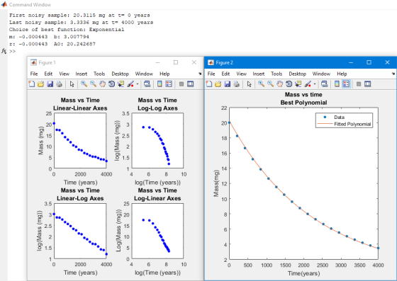
subplot(2,2,1)
plot((t),(A_Noisy),'b.','markersize',15)
xlabel('Time (years)')
ylabel('Mass (mg)')
title({'Mass vs Time';'Linear-Linear Axes'})
ylim([0,25])
subplot(2,2,2)
plot(log(t),log(A_Noisy),'b.','markersize',15)
xlabel('log(Time (years))')
ylabel('log(Mass (mg))')
title({'Mass vs Time';'Log-Log Axes'})
ylim([1,3.5])
subplot(2,2,3)
plot((t),log(A_Noisy),'b.','markersize',15)
xlabel('Time (years)')
ylabel('log(Mass (mg))')
ylim([1,3.5])
title({'Mass vs Time';'Linear-Log Axes'})
subplot(2,2,4)
plot(log(t),(A_Noisy),'b.','markersize',15)
xlabel('log(Time (years))')
ylabel('Log(Mass (mg))')
ylim([0,25])
title({'Mass vs Time';'Log-Linear Axes'})
%from the subplots, we see that the exponential function is the best fit, as it is the closest to a straight line
fprintf('Choice of best function: Exponential\n')

%%
%c
P=polyfit(t,log(A_Noisy),1);
m=P(1);
b=P(2);
fprintf('m: %.6f b: %.6f\n',m,b)

%%
%d
r_n=m;
A0_n=exp(b);
fprintf('r: %.6f A0: %.6f\n',r_n,A0_n)

%%
%e
t_new=0:1:4000;
figure
plot(t,A,'.','markersize',15)
hold on
plot(t_new,A0_n*exp(r_n*t_new))
legend('Data','Fitted Polynomial')
title({'Mass vs time';'Best Polynomial'})
xlabel('Time(years)')
ylabel('Mass(mg)')