Step 1:
Open the file named
e06ch11_grader_h1_Loans.xlsx. Save the file with the name
e06ch11_grader_h1_Loans_LastFirst.

Step 2:
Select cell C4 in the LoanAnalysis
worksheet and calculate the annual percentage rate for Loan Option
1. The formula is =RATE(C5,-C3,C2)*12.

Now, Format the cell as Percentage
with 2 decimal places.

Select the cell C4 then click on the
percentage as shown in the above image. After that, increase
decimal points by clicking on the increase decimal two times.
Step 3:
In cell 6, insert a formula by
selecting the insert function. A new window will be opened when the
insert function is selected. In the insert function window, select
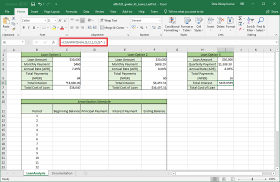
‘All’ in the category and select ‘CUMIPMT’ and then click ok.

The function arguments window will
be opened. In the function arguments window, scroll down to enter
the type. The type is 0. Enter the remaining values as specified in
the screenshot and then press ok. Reference cell C5 for the
end_period argument.

After clicking ok, the value will be
shown in the cell C6. To make sure the value is positive, multiply
the value with -1.

Format the cell as Currency.

The step3 can be directly done using
the formula,
=CUMIPMT($C4/12,$C5,$C2,1,$C5,0)*-1
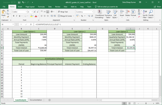
Step 4:
In cell C7, calculate the total cost
of the loan by adding the loan amount in cell C2 to the cumulative
interest amount in cell C6.
The formula is =(C2+C6).

Step 5:
In cell F3, calculate the end of the
period monthly payment for Loan Option 2 using the formula
=PMT($F4/12,$F5,$F2)

The monthly payment cannot be
negative. So, multiply the formula with -1. Now, the formula is
=PMT($F4/12,$F5,$F2)*-1.

Now, format the cell by right
clicking on cell F3. Select Format cells and then change the
currency. Select ‘$ English (United States)’ in the symbol. The
number of decimal places be 2.

Click on ok to see the result.

Step 6:
In cell F6, calculate the total
cumulative interest that would be paid throughout the life of the
loan if payments were made at the end of the periods.
The formula is
=CUMIPMT($F4/12,$F5,$F2,1,$F5,0).

Multiply the formula with -1 to make
sure that the result is positive.
Now, the formula is
=CUMIPMT($F4/12,$F5,$F2,1,$F5,0)*-1.

Now, format the cell F6 as currency.
Right click on the cell F6 and select format cells.

Step 7:
In cell F7, calculate the total cost
of the loan by adding the loan amount in cell F2 to the cumulative
interest amount in cell F6.
The formula is =(F2+F6).

Increase two decimal points in the
cell F7. It can be done by clicking two times on the increase
decimal icon as shown in the following image.

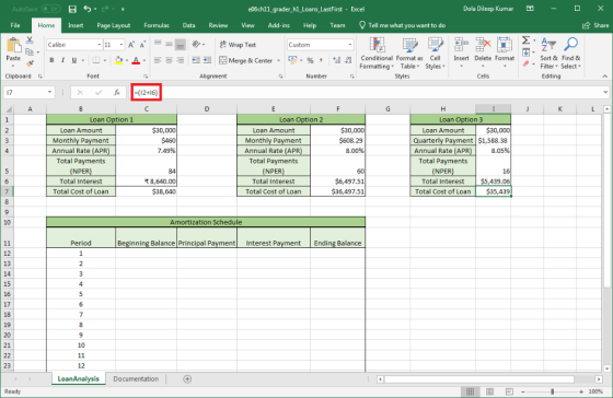
Step 8:
In cell I5, calculate the total
number of quarterly payments required to pay off Loan Option 3 if
payments are made at the end of the period.
The formula is
=NPER(I4/4,I3,I2).

The value of I5 should be positive.
Multiply with -1 to the value of I5.

Now decrease the decimal points to
0. It can be done by clicking on the decrease decimal icon 6
times.

Step 9:
In cell I6, calculate the total
cumulative interest that would be paid throughout the life of the
loan if payments were made at the end of the periods. Reference
cell I5 for the end_period argument.
The formula is
=CUMIPMT(I4/4,I5,I2,1,I5,0).

The value obtained is negative.
Multiply the value with -1.
The formula is
=CUMIPMT(I4/4,I5,I2,1,I5,0)*-1.
Convert the value to currency. It
can be done by right clicking on the cell and select format
cells.

By clicking on ok, the result is as
follows:
Step 10:
In cell I7, calculate the total cost
of the loan by adding the loan amount in cell I2 to the cumulative
interest amount in cell I6.
The formula is =(I2+I6).
Format the cell as follows:

Click on ok to apply the
changes.

Step 11:
In cell C12, enter a formula that
refers to the Loan Amount for Loan Option 3.
The formula is =I2.

Now, decrease the decimal points by
clicking on the decrease decimal.

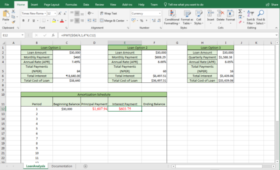
Step 12:
In cell D12, enter a function to
calculate the first principal payment.
The formula is
=PPMT($I$4/4,1,4*4,C12).
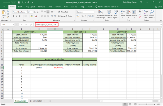
Format the cell as Currency with 2
decimal places.

By clicking on ok, the result is as
follows:

Step 13:
In cell E12, enter a function to
calculate the first interest payment.
=IPMT($I$4/4,1,4*4,C12)

Format the cell as Currency with 2
decimal places.
Step 14:
In cell F12, enter a formula to
calculate the first ending balance.
The formula is =C12+D12.

Format the cell as Currency with 2
decimal places.

Click on ok to see the result.

Step 15:
In cell C13, enter a formula that
refers to the ending balance in cell F12.
The formula is =F12.

Copy the formulas of D12, E12, F12
to D13, E13, F13.
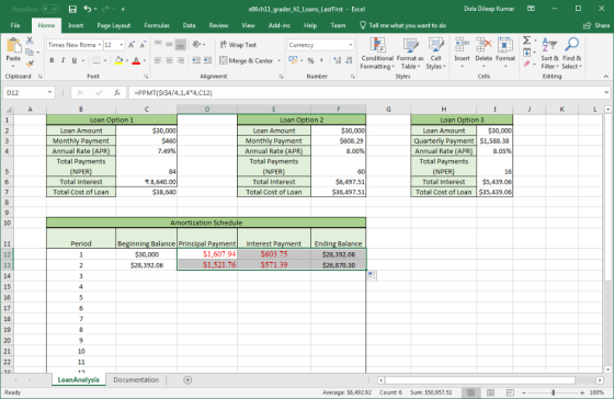
Select the cells from C13 to F13.
Drag the cells up to F35.

Step 16:
Save the worksheet as suggested.
Save As Info New Desktop Recent Open e06ch11 grader hl Loans LastFirst ESave Excel Workbook (dsx) Save OneDrive More options.. Save As This PC Name Date modified Print e06ch11 grader_h1_Loans_LastFirst.xlsx X 07-06-2019 12:38 Add a Place Share Export Browse Publish Close Account Feedback Options
Page Layout Formulas Tell me what you want to do File Home Insert Data Review View Add-ins Help Team Share 11A A = Wrap Text Calibri General BIU Insert Delete Format Paste Merge & Center Conditional Format as Cell Sort & Find & Filter Select A E7 Table Styles Formatting Clipboard r Number Styles Cells Editing Font Alignment = RATE ( C5 , - C3 ,C2)*12 C4 Formula Bar I A P D G K Loan Option 1 Loan Option 3 1 Loan Option 2 $30,000 $30,000 $30,000 Loan Amount 2 Loan Amount Loan Amount $460 0.074899846 Quarterly Payment $1,588.38 8.05% Monthly Payment Monthly Payment 3. Annual Rate (APR) Annual Rate (APR) 8.00% Annual Rate (APR) 4 Total Payments Total Payments Total Payments 5 (NPER) (NPER) (NPER) 84 60 Total Interest Total Interest Total Interest 6 7 Total Cost of Loan Total Cost of Loan Total Cost of Loan 10 Amortization Schedule Ending Balance Beginning Balance Principal Payment 11 Period Interest Payment 12 1 13 14 15 16 5 17 6 18 19 20 21 10 22 11 LoanAnalysis Documentation
Tell me what you want to do File Home Insert Page Layout Formulas Data Review View Add-ins Help Team Share 11 A A ab Wrap Text Calibri Percentage 6 Insert Delete Format Paste BIU Sort & Find & A == EE Merge & Center Conditional Format as Cell Formatting Table Styles Filter Select Editing Clipboard Font Alignment Number Styles Cells = RATE ( C5 , - C3 ,C2 ) *12 C4 D A G K 1 Loan Option 1 Loan Option 2 Loan Option 3 $30,000 oon'oce $460 $30,000 $30,000 2 Loan Amount Loan Amount Loan Amount Quarterly Payment $1,588.38 Monthly Payment Annual Rate (APR) Monthly Payment 3 8.00% Annual Rate (APR) 7,49% Annual Rate (APR) 8.05% 4 Total Payments Total Payments Total Payments (NPER) Total Interest (NPER) (NPER) 5 84 60 Total Interest Total Interest 6 Total Cost of Loan Total Cost of Loan 7 Total Cost of Loan 8 Amortization Schedule 10 Beginning Balance Principal Payment Period Interest Payment Ending Balance 11 12 1 13 14 15 16 17 18 19 20 21 10 22 11 LoanAnalysis Documentation +
Formulas Tell me what you want to do LShare File Home Insert Page Layout Data Review View Add-ins Help Team a Define Name Trace Precedents Show Formulas Trace Dependents Error Checking Σ A ED Use in Formula Calculation AutoSum Recently Financial Logical Text Date 8 Lookup & Math & Time Reference Trig Functions Insert More Name Watch Remove Arrows Evaluate Formula Create from Selection Function Used Manager Window Options Defined Names Function Library Formula Auditing Calculation Ce A C D I K H X- Insert Function 1. Loan Option 1 Loan Option 3 $30,000 Loan Amount $30,000 2. Loan Amount Search for a function: $460 Monthly Payment Quarterly Payment $1,588.38 Annual Rate (APR) 3 Type a brief description of what you want to do and then click Go Go 8.05 % Annual Rate (APR) 7,49% Total Payments (NPER) Total Payments (NPER) Or select a category: All 84 5 Select a function: Total Interest Total Interest 6 CUBERANKEDMEMBER Total Cost of Loan Total Cost of Loan 7 CUBESET UN 8 CHREVAL 9 CUMIPMT Amot 10 APRINC DATE CUMIPMT(rate,nper,pv,start period,end_period,type) Beginning Balance Pri Period 11 Returns the cumulative interest paid between two periods. 12 13 14 15 Help on this function OK Cancel 16 6 17 18 19 20 21 10 11 22 LoanAnalysis Documentation
Share Formulas Tell me what you want to do File Home Insert Page Layout Data Review View Add-ins Help Team Define Name fx Trace Precedents Show Formulas ? ... Trace Dependents Error Checking Use in Formula Calculation AutoSum Recently Financial Logical Used Text Date 8 Lookup & Math & Time Reference Insert More Name Watch ManagerCreate from Selection Remove Arrows Evaluate Formula Trig Functions window Function Formula Auditing Calculation Function Library Defined Names =CUMIPMT($C4/12, $C5, $ C2,1,$C5,0) CUMIPMT B A C E G H I J K 1 Loan Option 1 Loan Option 3 Amount Function Arguments $30,000 2 Loan Amount rly Payment $1,588.38 Rate (APR) Payments NPER) Interest Monthly Payment 3 CUMIPMT 8.05% Annual Rate (APR) Rate =0.006241654 sC4/12 Total Payments Nper SC5 =84 (NPER) =30000 Pv SC2 ,$C5,$C2,1,$C 6 Total Interest Start period 1 1 ost of Loan 7 Total Cost of Loan 84 End period SCs 8 = 8640 Returns the cumulative interest paid between two periods 10 End period s the last period in the calculation. Period 11 Beginning Ba 12 1 13 2 Formula result 8640 3 14 Help on this functioni Cancel OK 15 4 16 5 17 18 19 20 21 10 22 11 .. Documentation LoanAnalysis |
e06ch11 grader hl_Loans_LastFirst Excel X AutoSave fr Dola Dileep Kumar Tell me what you want to do LShare File Home Insert Page Layout Formulas Data Review View Add-ins Help Team EDefine Name 15Show Formulas fx Trace Precedents ? Use in Formula Trace DependentsError Checking ... Calculation AutoSum Recently Financial Logical Text Date & Lookup & Math & Trig Insert More Name Remove Arrows Evaluate Formula Manager Create from Selection Used Time Reference Function Functions Window Options Formula Auditing Defined Names Calculation Function Library =CUMIPMT($C4 /12,$C5, $C2,1, $C5,0)*-1 > f C6 A C D E F G H K Loan Option : Loan Option 3 1 Loan Option $30,000 $460 7.49% $30,000 $1,588.38 8.05 % $30,000 2 Loan Amount Loan Amount Loan Amount Monthly Payment Monthly Payment Quarterly Payment Annual Rate (APR) 3 Annual Rate (APR) 8.00% Annual Rate (APR) Total Payments Total Payments Total Payments (NPER) Total Interest (NPER) 5 84 60 (NPER) 8640 Total Interest Total Interest Total Cost of Loan Total Cost of Loan 7 Total Cost of Loan 8 10 Amortization Schedule Beginning Balance Principal Payment Ending Balance Period Interest Payment 11 12 1 13 2 14 15 4 16 5 17 6 18 7 19 20 10 21 1 22 LoanAnalysis Documentation +100% Ready
AutoSave O e06ch11 grader hl_Loans_LastFirst Excel X Dola Dileep Kumar Tell me what you want to do LShare File Home Insert Page Layout Formulas Data Review View Add-ins Help Team 11-A A Calibri abWrap Text Currency Insert Delete Format Conditional Format Paste Cel Sort & Find & B IU A Merge & Center EE Filter Select Formatting Table Styles Clipboard Styles Cells Editing Font Alignment Number =CUMIPMT($C4/12,$C5, $C2, 1, $C5, 0)*-1 C6 K A C D E G H Loan Option: Loan Option 2 Loan Option 3 1 $30,000 $460 7.49% $30,000 $30,000 2 Loan Amount Loan Amount Loan Amount Monthly Payment Monthly Payment Quarterly Payment $1,588.38 Annual Rate (APR) 3 8.05 % 8.00% Annual Rate (APR) Annual Rate (APR) Total Payments Total Payments Total Payments (NPER) Total Interest (NPER) 5 84 60 (NPER) Total Interest Total Interest 8.640.00 Total Cost of Loan 7 Total Cost of Loan Total Cost of Loan 8 10 Amortization Schedule Beginning Balance Principal Payment Ending Balance Period Interest Payment 11 12 1 13 2 14 15 4 16 5 17 6 18 7 19 20 10 21 1 22 LoanAnalysis Documentation +100% Ready WE%
AutoSave O X e06ch11 grader hl_Loans_LastFirst Excel Dola Dileep Kumar Tell me what you want to do LShare File Home Insert Page Layout Formulas Data Review View Add-ins Help Team Calibri 11 A A Wrap Text Custom Insert Delete Format Paste B IU A Conditional Format Cell Sort & Find & Merge & Center- EE % Filter Select Formatting Table Styles Clipboard Font Styles Cells Editing Alignment Number =(C2+C6) C7 K A C D E G H Loan Option 2 Loan Option 3 1 Loan Option 1 $30,000 $460 7.49% $30,000 $30,000 2 Loan Amount Loan Amount Loan Amount Monthly Payment Monthly Payment Quarterly Payment $1,588.38 Annual Rate (APR) 3 8.05 % 8.00% 4 Annual Rate (APR) Annual Rate (APR) Total Payments Total Payments Total Payments (NPER) Total Interest 84 (NPER) 60 (NPER) Total Interest Total Interest 6 8.640,00 $38,640 Total Cost of Loan Total Cost of Loan Total Cost of Loan 7 8 10 Amortization Schedule Beginning Balance Principal Payment Ending Balance Period Interest Payment 11 12 1 13 2 14 15 4 16 5 17 6 18 7 19 20 10 21 1 22 LoanAnalysis Documentation +100% Ready WE%
AutoSave O X e06ch11 grader hl_Loans_LastFirst Excel Dola Dileep Kumar Tell me what you want to do LShare File Home Insert Page Layout Formulas Data Review View Add-ins Help Team Calibri |11 A A Wrap Text Currency Insert Delete Format Paste A. Merge & Center- Conditional Format Cell Sort & Find & B IU E Filter Select Formatting Table Styles Alignment Clipboard Styles Cells Editing Font Number =PMT($F4/12,$F5, $F2) F3 K A C C E G H Loan Option 3 1 Loan Option 1 Loan Option 2 $30,000 $460 7.49% $30,000 $30,000 2 Loan Amount Loan Amount Loan Amount Monthly Payment Monthly Payment 3. -608.29 Quarterly Payment $1,588.38 Annual Rate (APR) 8.05 % Annual Rate (APR) 8.00% 4 Annual Rate (APR) Total Payments Total Payments Total Payments (NPER) Total Interest 84 (NPER) 60 (NPER) 8,640.00 Total Interest Total Interest 6 Total Cost of Loan $38,640 Total Cost of Loan Total Cost of Loan 7 8 10 Amortization Schedule Beginning Balance Principal Payment Ending Balance 11 Period Interest Payment 12 1 13 2 14 15 4 16 5 17 6 18 7 19 20 10 21 1 22 LoanAnalysis Documentation +100% Ready WE%
AutoSave O X e06ch11 grader hl_Loans_LastFirst Excel Dola Dileep Kumar Tell me what you want to do LShare File Home Insert Page Layout Formulas Data Review View Add-ins Help Team 11 A A Calibri ab Wrap Text Currency Insert Delete Format Paste A. Merge & Center- Conditional Format Cell Sort & Find & B IU E Filter Select Formatting Table Styles Clipboard Styles Cells Editing Font Alignment Number =PMT($F4/12,$F5, $F2) *-1 f F3 K A C E G H Loan Option 2 Loan Option 3 1 Loan Option 1 $30,000 $460 7.49% $30,000 $30,000 2 Loan Amount Loan Amount Loan Amount Monthly Payment Monthly Payment #608.29 3. $1,588.38 8.05 % Quarterly Payment 8.00% Annual Rate (APR) 4 Annual Rate (APR) Annual Rate (APR) Total Payments Total Payments Total Payments (NPER) Total Interest 84 (NPER) 60 (NPER) Total Interest 8,640.00 Total Interest 6 Total Cost of Loan $38,640 Total Cost of Loan Total Cost of Loan 7 8 10 Amortization Schedule Beginning Balance Principal Payment Ending Balance 11 Period Interest Payment 12 1 13 2 14 15 4 16 5 17 6 18 7 19 20 10 21 1 22 LoanAnalysis Documentation +100% Ready WE%
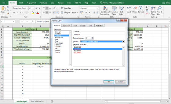
Share Formulas Review Add-ins Tell me what you want to do File Home Insert Page Layout Data View Help Team 11 A A ab Wrap Text Calibri Currency EE E Paste Conditional Format as Cell Insert Delete Format Sort & Find & Filter Select Merge & Center BIU Formatting Table Styles Number Styles Alianment Cells Editing Clipboard Font Format Cells PMT($F4/12,$F5, F3 Number Alignment Font Border Fill Protection A C K Sategory: on 3 1 Loan Option 1 Sample General $30,000 $30,000 2 Loan Amount $608.29 Currence $460 Monthly Payment $1,588.38 3. Accounting Decimal places: 2 Annual Rate (APR) 7.49% .05% 4 Time Percentage Symbol S English (United States) Total Payments 84 8,640.00 5 (NPER) numbers: Scientific 6 Total Interest Text $1,234.10 -$1.234.10 -51,234.10 Total Cost of Loan $38,640 7 Custom 8 9 10 Amorti Period Beginning Balance Pring 11 12 1 Currency formats are used for general monetary values. Use Accounting formats to align decimal points in a column. 13 14 15 16 17 Cancel OK 18 19 20 21 10 22 11 LoanAnalysis Documentation WE
AutoSave O X e06ch11 grader hl_Loans_LastFirst Excel Dola Dileep Kumar Tell me what you want to do LShare File Home Insert Page Layout Formulas Data Review View Add-ins Help Team 11-A A Calibri Wrap Text Currency Insert Delete Format Paste Conditional Format Cell Sort & Find & B IU A Merge & Center- E Filter Select Formatting Table Styles Clipboard Styles Cells Editing Font Alignment Number =PMT($F4/12, $F5, $F2) *-1 F3 K A C D E G H Loan Option 3 1 Loan Option 1 Loan Option 2 $30,000 $460 7.49% $30,000 $30,000 2 Loan Amount Loan Amount Loan Amount Monthly Payment Monthly Payment 3. Quarterly Payment $1,588.38 Annual Rate (APR) $608.29 8.05 % Annual Rate (APR) 8.00% 4 Annual Rate (APR) Total Payments Total Payments Total Payments (NPER) Total Interest 84 (NPER) 60 (NPER) 8,640.00 Total Interest Total Interest 6 Total Cost of Loan $38,640 Total Cost of Loan Total Cost of Loan 7 8 10 Amortization Schedule Beginning Balance Principal Payment Ending Balance 11 Period Interest Payment 12 1 13 2 14 15 4 16 5 17 6 18 7 19 20 10 21 1 22 LoanAnalysis Documentation +100% Ready WE%
AutoSave O X e06ch11 grader hl_Loans_LastFirst Excel Dola Dileep Kumar Tell me what you want to do LShare File Home Insert Page Layout Formulas Data Review View Add-ins Help Team Calibri 11 A A ab Wrap Text General Insert Delete Format Paste A. Merge & Center Conditional Format Cell Sort & Find & B IU E Filter Select Formatting Table Styles Clipboard Styles Cells Editing Font Alignment Number =CUMIPMT($F4/12, $F5, $ F2, 1,$F5,0) F6 K A C E G H Loan Option 3 1 Loan Option 1 Loan Option 2 $30,000 $460 7.49% $30,000 $30,000 2 Loan Amount Loan Amount Loan Amount Monthly Payment Monthly Payment Quarterly Payment $1,588.38 Annual Rate (APR) $608.29 3 8.05 % Annual Rate (APR) 8.00% Annual Rate (APR) Total Payments Total Payments Total Payments (NPER) Total Interest 84 (NPER) 5 60 (NPER) Total Interest 8,640.00 Total Interest -6497.509719 Total Cost of Loan $38,640 7 Total Cost of Loan Total Cost of Loan 8 10 Amortization Schedule Beginning Balance Principal Payment Ending Balance Period Interest Payment 11 12 1 13 2 14 15 4 16 5 17 6 18 7 19 20 10 21 1 22 LoanAnalysis Documentation +100% Ready WE%
AutoSave O X e06ch11 grader hl_Loans_LastFirst Excel Dola Dileep Kumar Tell me what you want to do LShare File Home Insert Page Layout Formulas Data Review View Add-ins Help Team Calibri 11-A A Wrap Text General Insert Delete Format Paste A Merge & Center- Conditional Format Cell Sort & Find & B IU E Filter Select Formatting Table Styles Clipboard Styles Cells Editing Font Alignment Number f =CUMIPMT($F4/12,$F5, $F2, 1,$F5,0) *-1 F6 K A C D E G H Loan Option 1 Loan Option 3 1 Loan Option 2 $30,000 $460 7.49% $30,000 $30,000 2 Loan Amount Loan Amount Loan Amount Monthly Payment Monthly Payment Quarterly Payment $1,588.38 Annual Rate (APR) $608.29 3 8.05 % Annual Rate (APR) 8.00% Annual Rate (APR) Total Payments Total Payments Total Payments (NPER) Total Interest 84 (NPER) 5 60 (NPER) Total Interest 8,640.00 Total Interest 6497.509719 Total Cost of Loan $38,640 7 Total Cost of Loan Total Cost of Loan 8 10 Amortization Schedule Beginning Balance Principal Payment Ending Balance Period Interest Payment 11 12 1 13 2 14 15 4 16 5 17 6 18 7 19 20 10 21 1 22 LoanAnalysis Documentation +100% Ready WE%
Page Layout Formulas Tell me what you want to do Add-ins Share File Home Insert Data Review View Help Team EAO 11A A ab Wrap Text Calibri Currency Sort & Find & Filter Select Conditional Format as Formatting Table Styles Paste BIU Cel Insert Delete Format A Merge & Center Clipboard Alignment Styles Cells Editing Font Number fe -CUMIPMT($F4/12,$F5,$F2,1,$F5,0)*-1 F6 G J A D E H K Loan Ontion 3 Loan Option 1 Loan Ontion 2 1 Format Cells $30,000 $460 $30,000 $1,588.38 Loan Amount Monthly Payment 3 Alignment Font Number Protection Border Fill 7.49% Annual Rate (APR) 8.05% 4 Total Payments Category Sample 5 (NPER) Total Interest 84 Number $6,497.51 8,640.00 6 Currency unting Decimal places: 2 $38.640 7 Total Cost of Loan Date Time 8 Symbol: SEnglish (United States) ge Fraction 9 Negative numbers: Scientific Amortiza -$1,234.10 S1.234.10 10 Text al Custom S1 234 10 Beginning Balance Princip 11 Period 12 1 13 14 4 15 16 Currency formats are used for general monetary values. Use Accounting formats to align decimal points in a column. 17 18 19 20 9 21 10 Cancel OK 22 11 23 17 LoanAnalysis Documentation 4 |I
Dola Dileep Kumar X AutoSave Off e06ch11 grader_h1_Loans_Last First - Excel Share File Home Insert Page Layout Formulas Data Review View Add-ins Help Team Tell me what you want to do 11A A Wrap Text Calibri Custom Conditional Forma Paste B IU A Cell Insert Delete Format .... Sort & Find & EMerge % Center Filter Select Styles Formatting Table Clipboard Font Alignment Cells Number Styles Editing =(F2+F6) F7 A C D P G H K. 1 Loan Option 1 Loan Option 2 Loan Option 3 $30,000 $460 $30,000 $30,000 2 Loan Amount Loan Amount Loan Amount Monthly Payment Annual Rate (APR) Quarterly Payment $1,588.38 Annual Rate (APR) Monthly Payment Annual Rate (APR) $608.29 3 7.49% 8.00% 8.05% 4. Total Payments Total Payments Total Payments 84 8,640.00 60 5 (NPER) (NPER) (NPER) $6,497.51 Total Interest 6 Total Interest Total Interest $36,498 7 Total Cost of Loan 8,640 Total Cost of Loan Total Cost of Loan 9 Amortization Schedule 10 Beginning Balance Principal Payment Period Ending Balance 11 Interest Payment 12 13 2 14 3 4 15 16 18 19 20 21 10 22 11 23 12 LoanAnalysis Documentation + 100 % Ready WE .
e06ch11_grader_h1_Loans_Last First-Excel Dola Dileep Kumar X AutoSave Off Tell me what you want to do Share File Home Insert Page Layout Formulas Data Review View Add-ins Help Team 11A A Wrap Text Calibri Custom Conditional Forma Paste B IU A Cell Insert Delete Format .... Sort & Find & EMerge Center Filter Select Styles Formatting Table Alignment Clipboard Font Cells Number Styles Editing = ( F2+F6) F7 A C D P G H K. Loan Option 2 1 Loan Option 1 Loan Option 3 $30,000 $460 Loan Amount $30,000 $30,000 2 Loan Amount Loan Amount Monthly Payment Annual Rate (APR) Quarterly Payment $1,588.38 Annual Rate (APR) Monthly Payment Annual Rate (APR) $608.29 3 7.49% 8.00% 8.05% 4. Total Payments Total Payments Total Payments 84 8,640.00 60 5 (NPER) (NPER) (NPER) $6,497.51 Total Interest 6 Total Interest Total Interest $36,497.51 7 Total Cost of Loan 8,640 Total Cost of Loan Total Cost of Loan 9 Amortization Schedule 10 Beginning Balance Principal Payment Period Ending Balance 11 Interest Payment 12 13 2 14 3 4 15 16 18 19 20 21 10 22 11 23 12 LoanAnalysis Documentation + 100 % Ready WE .
Dola Dileep Kumar X AutoSave Off e06ch11-grader_h1_Loans_Last First- Excel Tell me what you want to do Share File Home Insert Page Layout Formulas Data Review View Add-ins Help Team 11 A A Wrap Text Calibri General Conditional Forma Insert Delete Format Paste B IU A Cell .... Sort & Find & EMerge % Center Filter Select Styles Formatting- Table Alignment Clipboard Font Cells Number Styles Editing =NPER ( 14 / 4 ,13 , 12) fi I5 A C P G H K. Loan Option 2 1 Loan Option 1 Loan Option 3 $30,000 $460 $30,000 $30,000 2 Loan Amount Loan Amount Loan Amount Monthly Payment Annual Rate (APR) Monthly Payment Annual Rate (APR) $608.29 Quarterly Payment $1,588.38 Annual Rate (APR) 3 7.49% 8.00% 8,05% 4 Total Payments Total Payments Total Payments 84 8,640.00 60 5 (NPER) (NPER) (NPER) -16.16845 $6,497.51 Total Interest 6 Total Interest Total Interest $36,497.51 Total Cost of Loan 8,640 Total Cost of Loan Total Cost of Loan 7 8 9 Amortization Schedule 10 Beginning Balance Principal Payment Period Ending Balance 11 Interest Payment 12 13 2 14 3 4 15 16 18 19 20 21 10 22 11 23 12 LoanAnalysis Documentation + 100 % Ready WES EAH
Dola Dileep Kumar X AutoSave Off e06ch11-grader_h1_Loans_Last First- Excel Tell me what you want to do Share File Home Insert Page Layout Formulas Data Review View Add-ins Help Team 11A A ab Wrap Text Calibri General Conditional Forma Insert Delete Format Paste B IU A Cell .... Sort & Find & EMerge % Center Filter Select Styles Formatting- Table Clipboard Font Alignment Cells Number Styles Editing =NPER ( 14 / 4,13 , 12)*-1 I5 A C P G H K. Loan Option 2 1 Loan Option 1 Loan Option 3 $30,000 $460 $30,000 $30,000 2 Loan Amount Loan Amount Loan Amount Monthly Payment Annual Rate (APR) Quarterly Payment $1,588.38 Annual Rate (APR) Monthly Payment Annual Rate (APR) $608.29 3 7.49% 8.00% 8,05% 4 Total Payments Total Payments Total Payments 84 8,640.00 60 5 (NPER) (NPER) (NPER) Total Interest 16.168449 $6,497.51 6 Total Interest Total Interest $36,497.51 Total Cost of Loan 8,640 Total Cost of Loan Total Cost of Loan 7 8 9 Amortization Schedule 10 Beginning Balance Principal Payment Period Ending Balance 11 Interest Payment 12 13 2 14 3 4 15 16 18 19 20 21 10 22 11 23 12 LoanAnalysis Documentation + 100 % Ready WE EAH
Dola Dileep Kumar X AutoSave Off e06ch11_grader_h1_Loans_Last First-Excel Tell me what you want to do Share File Home Insert Page Layout Formulas Data Review View Add-ins Help Team 11A A ab Wrap Text Calibri Number 0Conditional Format a Styles Insert Delete Format Paste B IU A Cell .... Sort & Find & EMerge Center Filter Select Formatting Table Alignment Clipboard Font Cells Number Styles Editing - NPER ( 14 / 4,13,12)-1 I5 D A C P G H K. Loan Option 2 1 Loan Option 1 Loan Option 3 $30,000 $460 $30,000 $30,000 2 Loan Amount Loan Amount Loan Amount Quarterly Payment $1,588.38 Annual Rate (APR) Monthly Payment Annual Rate (APR) Monthly Payment Annual Rate (APR) $608.29 3 7.49% 8.00% 8.05% 4 Total Payments Total Payments Total Payments 84 8,640.00 60 16 5 (NPER) (NPER) (NPER) $6,497.51 6 Total Interest Total Interest Total Interest $36,497.51 Total Cost of Loan 8,640 Total Cost of Loan Total Cost of Loan 7 8 9 Amortization Schedule 10 Beginning Balance Principal Payment Period Ending Balance 11 Interest Payment 12 13 2 14 3 4 15 16 18 19 20 21 10 22 11 23 12 LoanAnalysis Documentation + 100 % Ready WE EAH
Dola Dileep Kumar X AutoSave Off e06ch11-grader_h1_Loans_Last First- Excel Tell me what you want to do Share File Home Insert Page Layout Formulas Data Review View Add-ins Help Team 11A A ab Wrap Text Calibri General Conditional Forma Insert Delete Format Paste B IU A Cell .... Sort & Find & EMerge % Center Filter Select Styles Formatting- Table Clipboard Font Cells Alignment Number Styles Editing -CUMIPMT(14/4,15,12,1, 15,0) l6 A C D G H K. Loan Option 2 1 Loan Option 1 Loan Option 3 $30,000 $460 $30,000 $30,000 2 Loan Amount Loan Amount Loan Amount Monthly Payment Annual Rate (APR) Total Payments Quarterly Payment $1,588.38 Annual Rate (APR) Monthly Payment Annual Rate (APR) $608.29 3 7.49% 8.00% 8.05% 4. Total Payments Total Payments 84 8,640.00 60 5 (NPER) (NPER) (NPER) 16 $6,497.51 6 Total Interest Total Interest Total Interest 5439,.06 $36,497.51 7 Total Cost of Loan 8,640 Total Cost of Loan Total Cost of Loan 8 9 Amortization Schedule 10 Beginning Balance Principal Payment Period Ending Balance 11 Interest Payment 12 13 2 14 3 4 15 16 18 19 20 21 10 22 11 23 12 LoanAnalysis Documentation + 100 % Ready WE
Dola Dileep Kumar X AutoSave Off e06ch11-grader_h1_Loans_Last First- Excel Tell me what you want to do Share File Home Insert Page Layout Formulas Data Review View Add-ins Help Team 11A A ab Wrap Text Calibri General Conditional Forma Insert Delete Format Paste B IU A Cell .... Sort & Find & % SMerge Center Filter Select Styles Formatting- Table Alignment Clipboard Font Cells Number Styles Editing -CUMIPMT(14/4,15, 12,1, 15,0) *- 1 fi l6 A C D G H K. Loan Option 2 Loan Option 3 1 Loan Option 1 $30,000 $460 $30,000 $30,000 2 Loan Amount Loan Amount Loan Amount Quarterly Payment $1,588.38 Annual Rate (APR) Monthly Payment Annual Rate (APR) Monthly Payment Annual Rate (APR) Total Payments $608.29 3 7.49% 8.00% 8.05% 4. Total Payments Total Payments 84 8,640.00 60 5 (NPER) (NPER) (NPER) 16 $6,497.51 Total Interest 6 Total Interest Total Interest 5439,0599 $36,497.51 7 Total Cost of Loan 8,640 Total Cost of Loan Total Cost of Loan 8 9 Amortization Schedule 10 Beginning Balance Principal Payment Period Ending Balance 11 Interest Payment 12 13 2 14 3 4 15 16 18 19 20 21 10 22 11 23 12 LoanAnalysis Documentation + 100 % Ready WE .
Tell me what you want to do File Share Home Insert Page Layout Formulas Data Review View Add-ins Help Team EAY 11 A A ab Wrap Text General Calibri Insert Delete Format Paste Merge & Center Conditional Format as Cell Sort & Find & A E BIU- Filter Select- Formatting Table Styles Clipboard r Font Alignment Number Styles Cells Editing fe =CUMIPMT(14/4,15,12,1, 15,0) * -1 A E G J K L oan Option 3 1 Loan Option 1 X- Format Cells $30,000 $30, mount 2 Loan Amount Monthly Payment Payment $1,588.38 ate (APR) yments ER) Number Alignment 7.4 Font Border Fil Protection Annual Rate (APR) 8.05% 4. Category Total Payments General Number Sample (NPER) 16 5 $5.439.06 8,640 $38, hterest Total Interest 6 5439.0599 Accounting Date Decimal places: 2 t of Loan 7 Total Cost of Loan Symbol: SEnglish (United States) 8 Percentage Fraction Negative numbers 9 ntifie -51,234.10 10 Special Custom -S1,234.10 $1.234.10 Period Beginning Bala 11 12 1 13 14 4 15 16 Currency formats are used for general monetary values. Use Accounting formats to align decimal points in a column. 17 18 7 19 20 9 Cancel OK 21 10 22 11 23 12 LoanAnalysis Documentation A
We were unable to transcribe this image
Dola Dileep Kumar X AutoSave Off e06ch11_grader_h1_Loans_Last First-Excel Share File Home Insert Page Layout Formulas Data Review View Add-ins Help Team Tell me what you want to do 11A A Wrap Text Calibri Custom Conditional Forma Insert Delete Format Paste B I U - A Cell .... Sort & Find & EMerge % Center Filter Select Styles Formatting Table Font Alignment Cells Clipboard Number Styles Editing fi (12+16) A C D P G H K. Loan Option 2 1 Loan Option 1 Loan Option 3 $30,000 $460 $30,000 $30,000 2 Loan Amount Loan Amount Loan Amount Monthly Payment Annual Rate (APR) Quarterly Payment $1,588.38 Annual Rate (APR) Monthly Payment Annual Rate (APR) $608.29 3 7.49% 8.00% 8.05% 4 Total Payments Total Payments Total Payments 84 8,640.00 60 16 5 (NPER) (NPER) (NPER) $6,497.51 Total Interest $5,439.06 6 Total Interest Total Interest $36,497.51 $35,439 7 Total Cost of Loan 8,640 Total Cost of Loan Total Cost of Loan 9 Amortization Schedule 10 Beginning Balance Principal Payment Period Ending Balance 11 Interest Payment 12 13 2 14 3 4 15 16 18 19 20 21 10 22 11 23 12 LoanAnalysis Documentation + 100 % Ready WE .
We were unable to transcribe this image
Dola Dileep Kumar X AutoSave Off e06ch11_grader_h1_Loans_Last First-Excel Share File Home Insert Page Layout Formulas Data Review View Add-ins Help Team Tell me what you want to do 11 A A ab Wrap Text Calibri Currency Conditional Forma Insert Delete Format Paste B I U - A Cell .... Sort & Find & EMerge Center Filter Select Styles Formatting Table Clipboard Font Alignment Number Styles Cell: Editing - ( 12+16 ) A C D P G K. L Loan Option 2 1 Loan Option 1 Loan Option 3 $30,000 $460 $30,000 $30,000 2 Loan Amount Loan Amount Loan Amount Quarterly Payment $1,588.38 Annual Rate (APR) Monthly Payment Annual Rate (APR) Monthly Payment Annual Rate (APR) $608.29 3 7.49% 8.00% 8.05% 4 Total Payments Total Payments Total Payments 84 8,640.00 60 5 (NPER) (NPER) (NPER) Total Interest 16 $6,497.51 $5,439.06 6 Total Interest Total Interest $36,497.51 Total Cost of Loan $35,439.06 7 Total Cost of Loan 8,640 Total Cost of Loan 9 Amortization Schedule 10 Beginning Balance Principal Payment Period Ending Balance 11 Interest Payment 12 13 2 14 3 4 15 16 18 19 20 21 10 22 11 23 12 LoanAnalysis Documentation + 100 % Ready WES EA
We were unable to transcribe this image
Dola Dileep Kumar X AutoSave Off e06ch11_grader_h1_Loans_Last First-Excel Tell me what you want to do Share File Home Insert Page Layout Formulas Data Review View Add-ins Help Team 11 A A Wrap Text Calibri Currency Conditional Forma Insert Delete Format Paste B I U - A Cell .... Sort & Find & EMerge Center Filter Select Styles Formatting Table Font Clipboard Alignment Number Styles Cell: Editing f C12 l2 A C D P G I K L Loan Option 1 Loan Option 2 1 Loan Option 3 $30,000 $460 $30,000 $30,000 2 Loan Amount Loan Amount Loan Amount Monthly Payment Annual Rate (APR) Monthly Payment Annual Rate (APR) $608.29 Quarterly Payment $1,588.38 Annual Rate (APR) 3 7.49% 8.00% 8.05% 4. Total Payments Total Payments Total Payments 84 8,640.00 60 5 (NPER) (NPER) (NPER) 16 $6,497.51 Total Interest $5,439.06 6 Total Interest Total Interest $36,497.51 Total Cost of Loan $35,439.06 $38,640 7 Total Cost of Loan Total Cost of Loan 8 9 Amortization Schedule 10 Period Beginning Balance Principal Payment Ending Balance 11 Interest Payment 12 $30,000 13 2 14 3 4 15 16 17 18 19 20 21 10 22 11 23 12 LoanAnalysis Documentation + 100 % Ready WE .
We were unable to transcribe this image
Tell me what you want to do File Home Insert Page Layout Formulas Data Review View Team Share Add-ins Help Times New Roma 12 A A Wrap Text Currency BIU EE Merge & Center Conditional Format as Paste Cell Insert Delete Format Sort & Find & A 00 Filter Select FormattingTable Styles Clipboard Editing Font Alignment Number Styles Cells X D12 Format Cells I A H Number Alignment Fill Font Border Protection Loan Option 1 Loan Option 3 Category $30,000 Quarterly Payment $1,588.38 Loan Amount 2. Loan Amount Sample General Monthly Payment 3 Number $1,607.94 8.05% Annual Rate (APR) Annual Rate (APR) 4 Accounting Decimal places: 2 Total Payments (NPER) Date Total Payments SEnglish (United States) Symbol: (NPER) 5 16 Percentage Negative numbers: -$1,234.10 $5,439.06 Fraction Total Interest Total Interest 6 Scientific Total Cost of Loan $35,439.06 Total Cost of Loan 7 $1 234.10 -S1,234.10 Special Custom 8 9 10 Period Beg 11 12 1 13 Currency formats are used for general monetary values. Use Accounting formats to align decimal points in a column. 14 15 4 16 17 OK Cancel 18 7 19 20 21 10 22 11 22 1* LoanAnalysis Documentation
Tell me what you want to do File Home Insert Page Layout Formulas Data Review View Add-ins Team Share Help 12 Times New Roma A A Wrap Text Currency Paste Conditional Format as Cell BIU »- A : Merge & Center Insert Delete Format Sort & Find & EE Filter Select Formatting Table Styles Alignment Clipboard Font Number Styles Cells Editing fox =PPMT($I$4/4,1,4*4,C12) D12 A C D F G J Loan Option 3 1 Loan Option 1 Loan Option 2 Loan Amount $30,000 $30,000 $30,000 2 Loan Amount Loan Amount Quarterly Payment $1,588.38 Annual Rate (APR) Monthly Payment $460 $608.29 3 Monthly Payment Annual Rate (APR) Annual Rate (APR) Total Payments 8.05% 7.49% 8.00% 4 Total Payments (NPER) Total Payments (NPER) 60 $6,497.51 (NPER) 5 84 16 $5,439.06 Total Cost of Loan $35,439.06 8,640.00 Total Interest Total Interest 6 Total Interest $38,640 Total Cost of Loan $36,497.51 7 Total Cost of Loan 8 9 10 Amortization Schedule Beginning Balance Principal Payment $1,607.94 Interest Payment Ending Balance 11 Period $30,000 12 1 13 14 15 4 16 17 6 18 19 20 21 10 22 11 22 17 LoanAnalysis Documentation
Dola Dileep Kumar X AutoSave Off e06ch11_grader_h1_Loans_Last First-Excel Share File Home Insert Page Layout Formulas Data Review View Add-ins Help Team Tell me what you want to do Times New Roma 12 A A ab Wrap Text Currency Conditional Forma Insert Delete Format Paste Cell .... Sort & Find & B I U A 圍Merge Center Filter Select Styles Formatting Table Alignment Clipboard Font Number Styles Cell: Editing =IPMT(SI$4/4,1,4*4,C12) fi E12 A C D G I K L Loan Option 1 1 Loan Option 2 Loan Option 3 $30,000 $30,000 $460 $30,000 2 Loan Amount Loan Amount Loan Amount Monthly Payment Annual Rate (APR) Monthly Payment Annual Rate (APR) $608.29 Quarterly Payment $1,588.38 Annual Rate (APR) 3 7.49% 8.00% 8.05% 4. Total Payments Total Payments Total Payments 84 8,640.00 60 5 (NPER) (NPER) (NPER) 16 $5,439.06 Total Cost of Loan $35,439.06 $6,497.51 Total Interest 6 Total Interest Total Interest $36,497.51 7 Total Cost of Loan 8,640 Total Cost of Loan 9 Amortization Schedule 10 Beginning Balance Principal Payment $1,607.94 Interest Payment Ending Balance Period 11 -603.75 $30,000 12 13 2 14 15 16 17 18 19 20 9 21 10 22 11 .. LoanAnalysis Documentation + 100 % Ready WE .
We were unable to transcribe this image
Tell me what you want to do Share Page Layout File Home Insert Formulas Data Review View Add-ins Help Team Times New Roma12 ab Wrap Text A A Currency Ep Paste Conditional Format as Cell Insert Delete Format Sort & Find & B IU . A Merge & Center Formatting Table Styles Filter Select Clipboard Editing Font Alignment Number Styles Cells =IPMT($I$4/4,1,4*4,C12) E12 D A F G H I J K Loan Option: Loan Option 2 1 Loan Option 3 $30,000 $460 7.49% $30,000 $30.000 2 Loan Amount Loan Amount Loan Amount Quarterly Payment $1,588.38 $608.29 Monthly Payment Monthly Payment 3 Annual Rate (APR) Annual Rate (APR) 8.00% Annual Rate (APR) 8.05% 4. Total Payments Total Payments Total Payments 84 8,640.00 (NPER) (NPER) 5 (NPER) 60 16 Total Interest Total Interest $6,497.51 Total Interest $5.439,06 6 Total Cost of Loan $35,439.06 $36,497.51 Total Cost of Loan $38,640 Total Cost of Loan 7 8 Amortization Schedule 10 Beginning Balance Principal Payment $1,607.94 Interest Payment Period Ending Balance 11 $30,000 $603.75 12 1 13 14 4 15 16 5 17 6 18 7 19 8 20 21 10 11 22 LoanAnalysis + Documentation
Dola Dileep Kumar X AutoSave Off e06ch11_grader_h1_Loans_Last First-Excel Share File Home Insert Page Layout Formulas Data Review View Add-ins Help Team Tell me what you want to do 11A A ab Wrap Text Calibri Currency Conditional Forma Insert Delete Format Paste B IU E- » - A Cell .... Sort & Find & EMerge Center Filter Select Styles Formatting Table Clipboard Font Alignment Number Styles Cell: Editing fi -C12+D12 F12 A C D P G I K L Loan Option 2 1 Loan Option 1 Loan Option 3 $30,000 $460 $30,000 $30,000 2 Loan Amount Loan Amount Loan Amount Monthly Payment Annual Rate (APR) Monthly Payment Annual Rate (APR) $608.29 Quarterly Payment $1,588.38 Annual Rate (APR) 3 7.49% 8.00% 8.05% 4. Total Payments Total Payments Total Payments 84 8,640.00 60 5 (NPER) (NPER) (NPER) 16 $5,439.06 $35,439.06 $6,497.51 Total Interest 6 Total Interest Total Interest $36,497.51 Total Cost of Loan 7 Total Cost of Loan 8,640 Total Cost of Loan 9 Amortization Schedule 10 Beginning Balance Principal Payment $1,607.94 Period Interest Payment $603.75 Ending Balance 11 $30,000 $28.392.06 12 13 2 14 15 16 17 18 19 20 9 21 10 22 11 .. LoanAnalysis Documentation + 100 % Ready WE .
We were unable to transcribe this image
Dola Dileep Kumar X AutoSave Off e06ch11_grader_h1_Loans_Last First-Excel Share File Home Insert Page Layout Formulas Data Review View Add-ins Help Team Tell me what you want to do 11 A A ab Wrap Text Calibri Currency Conditional Forma Insert Delete Format Paste B IU - A Cell .... Sort & Find & EMerge Center Filter Select Styles Formatting Table Clipboard Font Alignment Number Styles Cell: Editing F12 =C12+D12 A C D P G I K L Loan Option 1 Loan Option 2 1 Loan Option 3 $30,000 $460 $30,000 $30,000 2 Loan Amount Loan Amount Loan Amount Monthly Payment Annual Rate (APR) Monthly Payment Annual Rate (APR) $608.29 Quarterly Payment $1,588.38 Annual Rate (APR) 3 7.49% 8.00% 8.05% 4. Total Payments Total Payments Total Payments 84 8,640.00 60 5 (NPER) Total Interest (NPER) (NPER) 16 $5,439.06 $35,439.06 $6,497.51 Total Interest 6 Total Interest $36,497.51 Total Cost of Loan 7 Total Cost of Loan 8,640 Total Cost of Loan 9 Amortization Schedule 10 Beginning Balance Principal Payment $1,607.94 Period Interest Payment $603.75 Ending Balance 11 $30,000 $28.392.06 12 13 2 14 15 16 17 18 19 20 9 21 10 22 11 .. LoanAnalysis Documentation + 100 % Ready WE .
Dola Dileep Kumar X AutoSave Off e06ch11_grader_h1_Loans_Last First-Excel Share File Home Insert Page Layout Formulas Data Review View Add-ins Help Team Tell me what you want to do 11A A Wrap Text Calibri Currency Conditional Forma Insert Delete Format Paste B IU Cell .... Sort & Find & A EMerge Center Filter Select Styles Formatting Table Clipboard Font Alignment Number Styles Cell: Editing F12 C13 A D P G I K L Loan Option 1 Loan Option 2 1 Loan Option 3 $30,000 $460 $30,000 $30,000 2 Loan Amount Loan Amount Loan Amount Monthly Payment Annual Rate (APR) $608.29 Quarterly Payment $1,588.38 Annual Rate (APR) 3 Monthly Payment Annual Rate (APR) 7.49% 8.00% 8.05% 4. Total Payments Total Payments Total Payments 84 8,640.00 60 5 (NPER) Total Interest (NPER) (NPER) 16 $5,439.06 Total Cost of Loan $35,439.06 $6,497.51 Total Interest 6 Total Interest $36,497.51 7 Total Cost of Loan 8,640 Total Cost of Loan 8 9 Amortization Schedule 10 Beginning Balance Principal Payment $1,607.94 Period Interest Payment $603.75 Ending Balance 11 $30,000 $28,392.06 12 $28,392.06 13 2 14 3 15 16 17 18 19 20 9 21 10 22 11 .. LoanAnalysis Documentation + 100 % Ready WE .
Dola Dileep Kumar X AutoSave Off e06ch11_grader_h1_Loans_Last First-Excel Share File Home Insert Page Layout Formulas Data Review View Add-ins Help Team Tell me what you want to do A A Times New Roma 12 ab Wrap Text Currency Conditional Forma Insert Delete Format Paste Cell .... Sort & Find & B I U A Merge Center Filter Select Styles Formatting Table Clipboard Alignment Fon Number Styles Cell: Editing =PPMT($I$4/4,1,4*4,C12) D12 A C D G I K L 1 Loan Option 1 Loan Option 2 Loan Option 3 $30,000 $460 $30,000 $30,000 2 Loan Amount Loan Amount Loan Amount Monthly Payment Annual Rate (APR) Monthly Payment Annual Rate (APR) $608.29 Quarterly Payment $1,588.38 Annual Rate (APR) 3 7.49% 8.00% 8.05% 4. Total Payments Total Payments Total Payments 84 8,640.00 60 5 (NPER) (NPER) (NPER) 16 $5,439.06 Total Cost of Loan $35,439.06 $6,497.51 Total Interest 6 Total Interest Total Interest $36,497.51 7 Total Cost of Loan 8,640 Total Cost of Loan 8 9 Amortization Schedule 10 Beginning Balance Principal Payment Period Interest Payment Ending Balance 11 $1,607.94 $603.75 $28,392.06 12 $30.000 $1,521.76 13 $571.39 $28,392.06 $26,870.30 2 14 15 16 17 18 19 20 9 21 10 22 11 .. LoanAnalysis Documentation Average: $8,492.92 Sum: $50.957.51 + 100 % Ready Count: 6 WE .
Tell me what you want to do Formulas File Home Insert Page Layout Data Review View Add-ins Help Team Cut |11 A A ab Wrap Text Currency QA1LOFYNu... rfbm Calibri ECopy Paste Conditional Format a BIU - A Bad Merge & Center. Normal Format Painter % -5 Formatting Table Clipboard Font Alignment Number C13 =F12 A P C D P G 1 Loan Option 1 Loan Option 2 Loan Option 3 $30,000 Quarterly Payment $1,588.38 $30,000 $460 Loan Amount Loan Amount $30,000 2 Loan Amount Monthly Payment Monthly Payment $608.29 3 Annual Rate (APR) 8.00% Annual Rate (APR) 7.49% Annual Rate (APR) 8.05% 4 Total Payments Total Payments (NPER) Total Payments (NPER) 84 (NPER) 16 5 60 $6,497.51 $36,497.51 8,640.00 $5,439.06 $35,439.06 Total Interest Total Interest Total Interest 6 $38,640 Total Cost of Loan 7 Total Cost of Loan Total Cost of Loan 8 Amortization Schedule 10 Beginning Balance Principal Payment $30,000 Ending Balance $28,392.06 11 Period Interest Payment $1,607.94 $603.75 12 1 $26,870.30 $28,392.06 $1,521.76 $571.39 13 $1,440.20 $1,363.00 $540.76 $26,870.30 $25,430.10 14 $511.78 $24,067.10 $22,777.15 4 $25,430.10 15 $484.35 $24,067.10 $1,289.95 16 5 $22,777.15 $1,220.81 $458.39 $21,556.34 17 $1,155.38 $1,093.45 $1,034.85 $433.82 $20,400.96 $21,556.34 18 $410.57 $20,400.96 $19,307.51 19 8 $19,307.51 $388.56 $18,272.66 20 C $17,293.28 $18,272.66 $979.38 $367.74 10 21 $926.89 $348.03 $17,293.28 $16,366.40 22 11 $877.21 $329.37 $16,366.40 $15,489.19 23 12 $15,489.19 $830.19 $311.72 $14,659.00 24 13 $14,659.00 $785.69 $295.01 $13,873.30 14 25 $13,129.72 $12,425.99 $743.58 $279.20 $13,873.30 26 15 $703.73 $264.24 16 $13,129.72 27 $12,425.99 $666.01 $250.07 $11,759.98 17 28 $11,759.98 $630.31 $236.67 $11,129.67 29 18 $596.53 $223.98 $11,129.67 $10,533.14 30 19 $564.56 $211.98 $9,968.59 20 $10,533.14 31 $9,968.59 $534.30 $200.62 $9,434.29 32 21 $189.87 $9,434.29 $505.66 $8,928.63 33 22 $478.56 $179.69 $8,928.63 $8,450.07 34 23 $452.91 $170.06 $7,997.16 $8,450.07 35 24 36


 Assume a note is signed loan is taken out) on January 1, 2020 for $45.000 at a 5.25% interest rate with sixty monthly payments beginning February 1, 2020 Determine the monthly payment. NOTE: Format Excel so that cell values are in currency with no cents (no decimal places). Show your answers with dollar signs and commas but no cents. For example: $1,111 The following information will be used for Questions 7. 10. Use Excel to solve the problem. Assume a...
 Excel is allowed!
For this lab, we will create a spreadsheet that allows somebody to type in a loan amount, interest rate, and length of the loan in years. The spreadsheet will then calculate the monthly payment required and the actual amount paid on the loan. First, setup your spreadsheet: • In Cell A1, put the label Loan Amount:. The corresponding value would be input in Cell B1. • In Cell A2, put the label Interest Rate:. The corresponding value...
Excel is allowed!
For this lab, we will create a spreadsheet that allows somebody to type in a loan amount, interest rate, and length of the loan in years. The spreadsheet will then calculate the monthly payment required and the actual amount paid on the loan. First, setup your spreadsheet: • In Cell A1, put the label Loan Amount:. The corresponding value would be input in Cell B1. • In Cell A2, put the label Interest Rate:. The corresponding value...
 please post with pictures of step by step solution
oject Description: u own five apartment complexes. You created a dataset listing the apartment numbers, apartment complex mes, as last remodeled. You want artments need to number of bedrooms, rental price, whether the apartment is occupied or not, and the date the apartment to insert some functions to perform calculations to help you decide which be remodeled. To focus on the apartments that need to be remodeled, you will use vanced...
please post with pictures of step by step solution
oject Description: u own five apartment complexes. You created a dataset listing the apartment numbers, apartment complex mes, as last remodeled. You want artments need to number of bedrooms, rental price, whether the apartment is occupied or not, and the date the apartment to insert some functions to perform calculations to help you decide which be remodeled. To focus on the apartments that need to be remodeled, you will use vanced...
 Instructions:
For the purpose of grading the project you are required to
perform the following tasks:
Step
Instructions
Points Possible
1
Download and open the file named
exploring_e07_grader_a1_Sales.xlsx, and then save the file
as exploring_e07_grader_a1_Sales_LastFirst,
replacing LastFirst with your name.
0
2
On the Sales worksheet, enter a date function in cell C8 to
calculate the number of years the first representative has worked
for your company. Copy the function to the range C9:C20.
7
3
On the Sales worksheet,...
Instructions:
For the purpose of grading the project you are required to
perform the following tasks:
Step
Instructions
Points Possible
1
Download and open the file named
exploring_e07_grader_a1_Sales.xlsx, and then save the file
as exploring_e07_grader_a1_Sales_LastFirst,
replacing LastFirst with your name.
0
2
On the Sales worksheet, enter a date function in cell C8 to
calculate the number of years the first representative has worked
for your company. Copy the function to the range C9:C20.
7
3
On the Sales worksheet,...
 Please show the steps
BoyuQuCh7CaseStudy - Excel File Insert Page Layout Formulas Data Review View Add-ins ACROBAT QuickBooks Tell me what you want to do Sign in Share Σ Autosum Calibri Fill Paste в ㅣ u . re. O . . _ Ξ_ 트트 분 Merge & Center. $. % , 'i..g Conditional Format as Cell Insert Delete Format Sort & Find & Filter Select Formatting Table Styles Clipboard Font Alignment Number Cells Editing E3 Input Area Calculations 2 Facility...
Please show the steps
BoyuQuCh7CaseStudy - Excel File Insert Page Layout Formulas Data Review View Add-ins ACROBAT QuickBooks Tell me what you want to do Sign in Share Σ Autosum Calibri Fill Paste в ㅣ u . re. O . . _ Ξ_ 트트 분 Merge & Center. $. % , 'i..g Conditional Format as Cell Insert Delete Format Sort & Find & Filter Select Formatting Table Styles Clipboard Font Alignment Number Cells Editing E3 Input Area Calculations 2 Facility...
 Requiremeht1 Complete the data table DATA Loan Amount Interest Rate Periods 35,000 6% Requirement 2 Using the present value of an ordinary annuity table, calculate the payment amount and complete the amortization schedule Use the effective interest amortization method. a. Calculate the loan payment by dividing the loan amount by the appropriate present value factor b. Round values to two decimal places. Calculate the interest expense in the third year as the loan payment minus the loan balance at the...
 Long-term notes payable amortization schedule Dana's Delivery Services is buying a van to help with deliveries. The cost of the vehicle is $42,000, the interest rate is 6%, and the loan is for three years. 6 The van is to be repaid in three equal installment payments. Payments are due at the end of each year. Requirements 1. Complete the data table. 2. Using the present value of an ordinary annuity table, calculate the payment amount and complete the amortization schedule. Use the effective...
 My library>CptS 111 home> 2.9: zyLab PA #1: Student Loan R oks zyBooks cat @Help/FAQ θ Mohammed Al Shukaili 2.9 zyLabPA#1:Student Loan RepaymentCalculator For this assignment you wil write a program to calculate the monthly payments required to pay back a student loan You vill need to prompt the user for the following values Annual interest rate (as a percentage) Number of years to repay loan . and display the output in a readable form. Output should include Amount of...
 Prepare an amortization schedule for a five-year loan of $38,000. The interest rate is 7% per year, and the loan calls for equal annual payments. (Do not round intermediate calculations. Enter all amount as positive value. Round the final answers to 2 decimal places. Leave no cells blank - be certain to enter "0" wherever required.) Beginning Total Payment Interest Payment Principal Payment Ending Balance Year Balance Nm in How much interest is paid in the third year? (Do not...