I need a python code for this problem and it should contain 9 plots.


Homework Answers
code:
import math
def y(t): # lambda function
if t<2:
return 0
elif t>2 && t<4:
return t-2
elif t>4 && t<6:
return 2
else:
a = 2*math.exp(-(t-6))
return a
def diffy(t): # differentiation of lambda function
if t<2:
return 0
elif t>2 and t<4:
return 1
elif t>4 and t<6:
return 0
else:
a = 2*(-(t-6))*math.exp(-(t-5))
return a
def integy(t): #integration of lambda function
if t < 2:
return 0
elif t > 2 and t < 4:
return (t**2 /2 - 2*t )
elif t > 4 and t < 6:
return 2*t
else:
a = 2*math.exp(-(t-6))/(-(t-6))
return a
#solving question 1
import matplotlib.pyplot as plt
import numpy as np
t = np.arange(0.,16.,0.5)
acceleration = []
for i in range(len(t)):
acceleration.append(y(t[i]))
velocity = [] # integration of acceleration = integy function
for i in range(len(t)):
velocity.append(integy(t[i]))
#print(acceleration)
#print(velocity)
position1 = [a*b for a,b in zip(velocity,t)]
positiion2 = [(1/2)a(b**2) for a,b in zip(acceleration,t)]
position = [a+b for a,b in zip(position1,positiion2)]
plt.plot(t,position,c='red',ls='',marker='*')
ax = plt.gca()
ax.set_ylim([0,10])
plt.title('Position vs time')
plt.xlabel('time')
plt.ylabel('position')
plt.show()
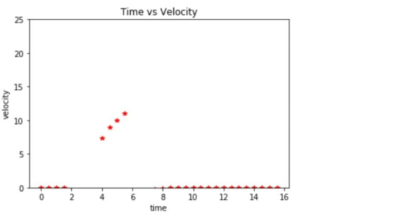
plt.plot(t,velocity,c='red',ls='',marker='*')
ax = plt.gca()
ax.set_ylim([0,25])
plt.title('Time vs Velocity')
plt.xlabel('time')
plt.ylabel('velocity')
plt.show()
plt.plot(t,acceleration,c='red',ls='',marker='*')
ax = plt.gca()
ax.set_ylim([0,5])
plt.title('Time vs Acceleration')
plt.xlabel('time')
plt.ylabel('accaeleration')
plt.show()
#Solving question2
t = np.arange(0.,16.,0.5)
velocity = []
for i in range(len(t)):
velocity.append(y(t[i]))
acceleration= [] # integration of acceleration = integy
function
for i in range(len(t)):
acceleration.append(integy(t[i]))
#print(acceleration)
#print(velocity)
position1 = [a*b for a,b in zip(velocity,t)]
positiion2 = [(1/2)a(b**2) for a,b in zip(acceleration,t)]
position = [a+b for a,b in zip(position1,positiion2)]
plt.plot(t,position,c='red',ls='',marker='*')
ax = plt.gca()
ax.set_ylim([0,500])
plt.title('Position vs time')
plt.xlabel('time')
plt.ylabel('position')
plt.show()
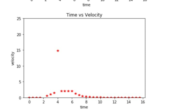
plt.plot(t,velocity,c='red',ls='',marker='*')
ax = plt.gca()
ax.set_ylim([0,25])
plt.title('Time vs Velocity')
plt.xlabel('time')
plt.ylabel('velocity')
plt.show()
plt.plot(t,acceleration,c='red',ls='',marker='*')
ax = plt.gca()
ax.set_ylim([0,50])
plt.title('Time vs Acceleration')
plt.xlabel('time')
plt.ylabel('accaeleration')
plt.show()
# solving question3
t = np.arange(0.,16.,0.5)
position = []
for i in range(len(t)):
position.append(y(t[i]))
velocity = [] # integration of acceleration = integy function
acceleration=[]
#print(acceleration)
#print(velocity)
acceleration= [2*(a/(t**2)) for a,b in zip(position,t)]
velocity = [2*a*b for a,b in zip(acceleration,position)]
velocity = [i**(1/2) for i in velocity]
plt.plot(t,position,c='red',ls='',marker='*')
ax = plt.gca()
ax.set_ylim([0,10])
plt.title('Position vs time')
plt.xlabel('time')
plt.ylabel('position')
plt.show()
plt.plot(t,velocity,c='red',ls='',marker='*')
ax = plt.gca()
ax.set_ylim([0,25])
plt.title('Time vs Velocity')
plt.xlabel('time')
plt.ylabel('velocity')
plt.show()
plt.plot(t,acceleration,c='red',ls='',marker='*')
ax = plt.gca()
ax.set_ylim([0,5])
plt.title('Time vs Acceleration')
plt.xlabel('time')
plt.ylabel('accaeleration')
plt.show();
SCREENSHOT;
![[2]: import math def y(t): if t<2: return elif t>2 && t<4: return t-2 elif t>4 && t<6: return 2 else: a = 2*math.exp(-(t-6))](http://img.homeworklib.com/questions/c5881880-bfad-11eb-acc1-b73e7c09ea40.png?x-oss-process=image/resize,w_560)
![[4]: def integy(t): if t < 2: return 0 elif t > 2 and t < 4: return (t**2 /2 - 2*t ) elif t > 4 and t < 6: return 2*t else: a](http://img.homeworklib.com/questions/c61fd6d0-bfad-11eb-a441-cb6c01649770.png?x-oss-process=image/resize,w_560)
![positiion2 = [(1/2)*a*(b**2) for a,b in zip(acceleration, t)] position = [a+b for a,b in zip(positioni, positiion2)] plt.plot](http://img.homeworklib.com/questions/c6d46600-bfad-11eb-bfeb-9127cea68cba.png?x-oss-process=image/resize,w_560)

![Time vs Acceleration accaeleration 2 4 6 8 time 10 12 14 16 [39]: #Solving question2 t = np.arange (0., 16.,0.5) velocity = [](http://img.homeworklib.com/questions/c859ea20-bfad-11eb-8d93-37b013779901.png?x-oss-process=image/resize,w_560)
![TPI LILI UCCELEIUL LUI #print(velocity) position1 = [a*b for a,b in zip(velocity,t)] positiion2 = [(1/2)*a*(b**2) for a,b in](http://img.homeworklib.com/questions/c8e951a0-bfad-11eb-bab2-ab4188c5c62d.png?x-oss-process=image/resize,w_560)

![Time vs Acceleration accaeleration 00 À 681021416 time [42]: # solving question3 t = np.arange(0.,16., 0.5) position = [] for](http://img.homeworklib.com/questions/ca96b3d0-bfad-11eb-9859-c3bb9cee1b18.png?x-oss-process=image/resize,w_560)
![acceleration= [2*(a){t**2)) for a, b in zip position,t)] velocity = [2*a*b for a, b in zip(acceleration, position)] velocity](http://img.homeworklib.com/questions/cb2ff1f0-bfad-11eb-9dea-798c38ec27a1.png?x-oss-process=image/resize,w_560)


Add Answer to:
I need a python code for this problem and it should contain 9
plots.
- Problem...
I need this project Manual and simulation solution
 An internal combustion engine slider-crank mechanism is shown in the figure. Crank AB rotates in selected clockwise positive direction as shown. Piston position is Y=AD. is angular position of the crank, is angular velocity of the crank, is angular acceleration of the crank. A-Analytical formulations part: 1) With the given parameters find analytical expressions for :a) Piston position, Y [mm]b) Piston velocity, [mm/s]c) Piston acceleration [mm/s2].(Show all the details of the derivations including your figure with given coordinate directions etc.) B-Computer Simulations part: 2) ...
Consider the Spring-Mass-Damper system: 17 →xt) linn M A Falt) Ffl v) Consider the following system...
 Consider the Spring-Mass-Damper system: 17 →xt) linn M A Falt) Ffl v) Consider the following system parameter values: Case 1: m= 7 kg; b = 1 Nsec/m; Fa = 3N; k = 2 N/m; x(0) = 4 m;x_dot(0)=0 m/s Case2:m=30kg;b=1Nsec/m; Fa=3N; k=2N/m;x(0)=2m;x_dot(0)=0m/s Use MATLAB in order to do the following: 1. Solve the system equations numerically (using the ODE45 function). 2. For the two cases, plot the Position x(t) of the mass, on the same graph (include proper titles, axis...
[1] CONSIDER THESE TWO Cases : 1. A ball moves in uniform circular motion. ...
[1] CONSIDER THESE TWO Cases : 1. A ball moves in uniform circular motion. (i) Sketch a two dimensional position plot of the functions x(t) and y(t). Extra credit: What type of plot is this? (5 points). (ii) On your plot, draw in five different velocity vectors at different times. (iii) Is there an acceleration ? Why or why not? 2. A ball moves in a straight line while its speed decreases. (i)...
Data Trial 1 Trial 2 Trial 3 Distance travelled by mass, S (m) [Same for each trial) 05 m 0.5 m 0...
 Data Trial 1 Trial 2 Trial 3 Distance travelled by mass, S (m) [Same for each trial) 05 m 0.5 m 0.5 m Total mass moved (M+m) (KG) 03284 .?'to. same in all trials Hanging mass (m) [different in each trial] Time between gates, t (sec) 14 It% |t2-O-68 t3 #0.99 d Experimental Acceleration, dexp (m/s) (use: S vot t ^at2) 4 165 mls try to make vo Theoretical Acceleration, athe (m/s2) (use: aINM+m Difference (%) mg 15.3 Task 1:...
modify this code is ready % Use ODE45 to solve Example 4.4.3, page 205, Palm 3rd...
 modify this code is ready
% Use ODE45 to solve Example 4.4.3, page 205, Palm 3rd
edition
% Spring Mass Damper system with initial displacement
function SolveODEs()
clf %clear any existing plots
% Time range Initial Conditions
[t,y] = ode45( @deriv, [0,2], [1,0] );
% tvals yvals color and style
plot( t, y(:,1), 'blue');
title('Spring Mass Damper with initial displacement');
xlabel('Time - s');
ylabel('Position - ft');
pause % hit enter to go to the next plot
plot( t, y(:,2), 'blue--');...
modify this code is ready
% Use ODE45 to solve Example 4.4.3, page 205, Palm 3rd
edition
% Spring Mass Damper system with initial displacement
function SolveODEs()
clf %clear any existing plots
% Time range Initial Conditions
[t,y] = ode45( @deriv, [0,2], [1,0] );
% tvals yvals color and style
plot( t, y(:,1), 'blue');
title('Spring Mass Damper with initial displacement');
xlabel('Time - s');
ylabel('Position - ft');
pause % hit enter to go to the next plot
plot( t, y(:,2), 'blue--');...
Please solve the problem below. I would really like to see work shown so I can understand the concepts and the things I...
 Please solve the problem below. I would really like to see work
shown so I can understand the concepts and the things I am doing
incorrectly.
|(1 point) A mass of 4 kg stretches a spring 40 cm. The mass is acted on by an external force of F(t) = 97 cos(0.5t) N and moves in a medium that imparts a viscous force of 4 N when the speed of the mass is 8 cm/s. If the mass is set...
Please solve the problem below. I would really like to see work
shown so I can understand the concepts and the things I am doing
incorrectly.
|(1 point) A mass of 4 kg stretches a spring 40 cm. The mass is acted on by an external force of F(t) = 97 cos(0.5t) N and moves in a medium that imparts a viscous force of 4 N when the speed of the mass is 8 cm/s. If the mass is set...
9. Consider the plant T(s)= A10and the given root locus plots. a. Which plot was generated...
 9. Consider the plant T(s)= A10and the given root locus plots. a. Which plot was generated for the plant with a proportional controller? (1) (2) (3) b. Which plot was generated for the plant with a pure integral controller? (1) (2) (3) c. Which plot was generated for the plant with a PI-controller? (1) (2) (3) d. What is the smallest time constant that closed-loop systems represented by plot (2) can have? s24+100 Which plot has the possibility of non-oscilating...
I want the math lab code for theses problems in a unique way
 I
want the math lab code for theses problems in a unique way
Theory A projectile is launched from point A up an incline plane that makes an angle of 10 with the horizontal. The mountain is 6,000 m high. Vo 10° Figure 1: Flightpath of a projectile. If we neglect the air resistance, the flight path of a projectile launched at an initial speed vo and an angle θ of departure relative to the horizontal is a parabola (see...
I
want the math lab code for theses problems in a unique way
Theory A projectile is launched from point A up an incline plane that makes an angle of 10 with the horizontal. The mountain is 6,000 m high. Vo 10° Figure 1: Flightpath of a projectile. If we neglect the air resistance, the flight path of a projectile launched at an initial speed vo and an angle θ of departure relative to the horizontal is a parabola (see...
Interactive Exercises 2.14: Acceleration and Velocity Plots (Monster RC Truck) A radio-controlled (RC) truck moves along...
 Interactive Exercises 2.14: Acceleration and Velocity Plots (Monster RC Truck) A radio-controlled (RC) truck moves along an x axis with an acceleration that depends on time in a manner shown in the graph in Interactive Fig. 2.14.1 below. At the instant0 the velocity of the truck is -1 m/s and its position is at the origin a (m/s) 0, 1 (s) 10 Interactive Figure 2.14.1: The acceleration versus time plot for an RC truck that moves on an axis. ▼...
Please I need help with question #7 C. 5. 9. 10. 11 Given the rate of...
 Please I need help with question #7
C. 5. 9. 10. 11 Given the rate of change of a quantity and its initial value explain how to find the value of at a future time 1 2 0. 6. What is the result of integrating a population growth rate between times I = a and 1 = b. where b > a? Basic Skills 7. Displacement and distance from velocity Consider the graph shown in the figure, which gives the...
Please I need help with question #7
C. 5. 9. 10. 11 Given the rate of change of a quantity and its initial value explain how to find the value of at a future time 1 2 0. 6. What is the result of integrating a population growth rate between times I = a and 1 = b. where b > a? Basic Skills 7. Displacement and distance from velocity Consider the graph shown in the figure, which gives the...
 Consider the Spring-Mass-Damper system: 17 →xt) linn M A Falt) Ffl v) Consider the following system parameter values: Case 1: m= 7 kg; b = 1 Nsec/m; Fa = 3N; k = 2 N/m; x(0) = 4 m;x_dot(0)=0 m/s Case2:m=30kg;b=1Nsec/m; Fa=3N; k=2N/m;x(0)=2m;x_dot(0)=0m/s Use MATLAB in order to do the following: 1. Solve the system equations numerically (using the ODE45 function). 2. For the two cases, plot the Position x(t) of the mass, on the same graph (include proper titles, axis...
 Data Trial 1 Trial 2 Trial 3 Distance travelled by mass, S (m) [Same for each trial) 05 m 0.5 m 0.5 m Total mass moved (M+m) (KG) 03284 .?'to. same in all trials Hanging mass (m) [different in each trial] Time between gates, t (sec) 14 It% |t2-O-68 t3 #0.99 d Experimental Acceleration, dexp (m/s) (use: S vot t ^at2) 4 165 mls try to make vo Theoretical Acceleration, athe (m/s2) (use: aINM+m Difference (%) mg 15.3 Task 1:...
 modify this code is ready
% Use ODE45 to solve Example 4.4.3, page 205, Palm 3rd
edition
% Spring Mass Damper system with initial displacement
function SolveODEs()
clf %clear any existing plots
% Time range Initial Conditions
[t,y] = ode45( @deriv, [0,2], [1,0] );
% tvals yvals color and style
plot( t, y(:,1), 'blue');
title('Spring Mass Damper with initial displacement');
xlabel('Time - s');
ylabel('Position - ft');
pause % hit enter to go to the next plot
plot( t, y(:,2), 'blue--');...
modify this code is ready
% Use ODE45 to solve Example 4.4.3, page 205, Palm 3rd
edition
% Spring Mass Damper system with initial displacement
function SolveODEs()
clf %clear any existing plots
% Time range Initial Conditions
[t,y] = ode45( @deriv, [0,2], [1,0] );
% tvals yvals color and style
plot( t, y(:,1), 'blue');
title('Spring Mass Damper with initial displacement');
xlabel('Time - s');
ylabel('Position - ft');
pause % hit enter to go to the next plot
plot( t, y(:,2), 'blue--');...
 Please solve the problem below. I would really like to see work
shown so I can understand the concepts and the things I am doing
incorrectly.
|(1 point) A mass of 4 kg stretches a spring 40 cm. The mass is acted on by an external force of F(t) = 97 cos(0.5t) N and moves in a medium that imparts a viscous force of 4 N when the speed of the mass is 8 cm/s. If the mass is set...
Please solve the problem below. I would really like to see work
shown so I can understand the concepts and the things I am doing
incorrectly.
|(1 point) A mass of 4 kg stretches a spring 40 cm. The mass is acted on by an external force of F(t) = 97 cos(0.5t) N and moves in a medium that imparts a viscous force of 4 N when the speed of the mass is 8 cm/s. If the mass is set...
 9. Consider the plant T(s)= A10and the given root locus plots. a. Which plot was generated for the plant with a proportional controller? (1) (2) (3) b. Which plot was generated for the plant with a pure integral controller? (1) (2) (3) c. Which plot was generated for the plant with a PI-controller? (1) (2) (3) d. What is the smallest time constant that closed-loop systems represented by plot (2) can have? s24+100 Which plot has the possibility of non-oscilating...
 I
want the math lab code for theses problems in a unique way
Theory A projectile is launched from point A up an incline plane that makes an angle of 10 with the horizontal. The mountain is 6,000 m high. Vo 10° Figure 1: Flightpath of a projectile. If we neglect the air resistance, the flight path of a projectile launched at an initial speed vo and an angle θ of departure relative to the horizontal is a parabola (see...
I
want the math lab code for theses problems in a unique way
Theory A projectile is launched from point A up an incline plane that makes an angle of 10 with the horizontal. The mountain is 6,000 m high. Vo 10° Figure 1: Flightpath of a projectile. If we neglect the air resistance, the flight path of a projectile launched at an initial speed vo and an angle θ of departure relative to the horizontal is a parabola (see...
 Interactive Exercises 2.14: Acceleration and Velocity Plots (Monster RC Truck) A radio-controlled (RC) truck moves along an x axis with an acceleration that depends on time in a manner shown in the graph in Interactive Fig. 2.14.1 below. At the instant0 the velocity of the truck is -1 m/s and its position is at the origin a (m/s) 0, 1 (s) 10 Interactive Figure 2.14.1: The acceleration versus time plot for an RC truck that moves on an axis. ▼...
 Please I need help with question #7
C. 5. 9. 10. 11 Given the rate of change of a quantity and its initial value explain how to find the value of at a future time 1 2 0. 6. What is the result of integrating a population growth rate between times I = a and 1 = b. where b > a? Basic Skills 7. Displacement and distance from velocity Consider the graph shown in the figure, which gives the...
Please I need help with question #7
C. 5. 9. 10. 11 Given the rate of change of a quantity and its initial value explain how to find the value of at a future time 1 2 0. 6. What is the result of integrating a population growth rate between times I = a and 1 = b. where b > a? Basic Skills 7. Displacement and distance from velocity Consider the graph shown in the figure, which gives the...
Most questions answered within 3 hours.
-
Where is the error in this code sequence?
String s1 = "Hello";
String s2 = "ello";...
asked 11 months ago -
Financial data for Joel de Paris, Inc., for last year
follow:
Joel de Paris, Inc.
Balance...
asked 11 months ago -
Consider this reaction:
Al2(SO4)3 (aq)+ BaCl3
(aq) Al2Cl6 (aq)- +
3BaSO4(s) . What is the...
asked 11 months ago -
Suppose that Savneet is considering increasing her
recent random sample from 20 car rentals to 40...
asked 11 months ago -
Trucks arrive at an unloading terminal at an average rate of 120
per hour.
Trucks arrive...
asked 11 months ago -
Why are methanol and ethanol completely soluble in water while
octanol is not very little soluble....
asked 11 months ago -
A facilities manager at a university reads in a research report
that the mean amount of...
asked 11 months ago -
When the CuSO4 is rehydrated by adding water to the anhydrous
compound, is this an endothermic...
asked 11 months ago -
A ray of sunlight is passing from diamond into crown glass; the
angle of incidence is...
asked 11 months ago -
A block of mass 0.249 kg is placed on top of a light, vertical
spring of...
asked 11 months ago -
how do the kidneys compensate in the presences of acidosis
a) trigger hyperventilate
b) reserve acid...
asked 11 months ago -
Question 501 pts
The rental rate of capital to the firm increases. Which of the
following...
asked 11 months ago