

Homework Answers
Main Code
%%%%%%%%%%%%%%%%%%%%%%%%%%%%%%%%%%%%%%%%%%%%%
close all,
clear all,
clc,
Fs=1000;
F=50;
T = 1/Fs;
L=10000;
t=(0:(L-1))*T;
ShowLength=150;
length(t)
d = 0.7*sin(2*pi*F*t);
Noise = rand(size(t)); %Full Scale Noise Input to Filter
x = d + 10*Noise;
subplot(5,1,1); plot(Fs*t(1:ShowLength),d(1:ShowLength)); grid on,
title('Original Clean Signal');
subplot(5,1,2); plot(Fs*t(1:ShowLength),Noise(1:ShowLength)); grid
on, title('Full Scale Noise Signal');
subplot(5,1,3); plot(Fs*t(1:ShowLength),x(1:ShowLength)); grid on,
title('Original Signal Corrupted with Full Scale Zero Mean Random
Noise');
Order=31;
h = fir1(Order,0.5); % FIR system to be identified
delta = 0.001; % LMS step size.
N= length(h);
DesiredSignal = filter(h,1,x)+ (Noise); % Desired signal at 10
times the Full scale Noise
[h,y] = mylms(x,DesiredSignal,delta,N,Fs,t);
subplot(5,1,4); plot(Fs*t(1:ShowLength),2*y(1:ShowLength)); grid
on, title('Filtered Signal');
%%%%%%%%%%%%%%%%%%%%%%%%%%%%%%%%%%%%%%%%%%%%%%%%%%
Function Code
%%%%%%%%%%%%%%%%%%%%%%%%%%%%%%%%%%%%%%%%%%%%%%%%%%%
function [h, y] = mylms(x,d,delta,N,Fs,t)
M = length(x);
h = zeros(1,N);
for n=N:M
x1 = x(n:-1:n-N+1);
y(n) = h*x1';
e = d(n)-y(n);
h=h+delta*e*x1;
end
end
%%%%%%%%%%%%%%%%%%%%%%%%%%%%%%%%%%%%%%%%%%%%%%%%%%%
As the step size decreases, the ASE decreases.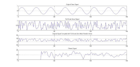
Add Answer to:
LMS project Using the notes discussed in class: Implementing the LMS Algorithm First generate some signals...
LMS project Using the notes discussed in class: Implementing the LMS Algorithm First generate some signals clear all c...
 LMS project Using the notes discussed in class: Implementing the LMS Algorithm First generate some signals clear all close al1: Generate signals for testing the LMS Algorithm 1000 Fs Sampling frequency Sample time 1/Fs 10000: = L Length of signal S Time vector (0:L-1) *T ; Sum of a 50 Hz sinusoid and a 120 Hz sinusoid 0.7 sin (2*pi*50*t); inuside X d+ 10 randn (size (t)); Sinusoids 5O0000000L plus noise fiqure (1) plot (Fs*t (1:150),x (1:1500)) title('Signal Corrupted with...
Question 4 (a) Find the DFT of the series x[n)-(0.2,1,1,0.2), and sketch the magnitude of the resulting spectral components [10 marks] (b) For a discrete impulse response, h[n], that is symmetric...
 Question 4 (a) Find the DFT of the series x[n)-(0.2,1,1,0.2), and sketch the magnitude of the resulting spectral components [10 marks] (b) For a discrete impulse response, h[n], that is symmetric about the origin, the spectral coefficients of the signal, H(k), can be obtained by use of the DFT He- H(k)- H-(N-1)/2 Conversely, if the spectral coefficients, H(k), are known (and are even and symmetrical about k-0), the original signal, h[n], can be reconstituted using the inverse DFT 1 (N-D/2...
[MATLAB Scriptfile task] Design N-band tone vocoder with a given figure (below) in MATLAB implementing the...
 [MATLAB Scriptfile task]
Design N-band tone vocoder with a given figure (below) in MATLAB
implementing the given script file(bands_cutoff). This program
should be able to process any sound(.wav) file. Then, graph the
band-passed signals and amplitude envelopes extracted(after
rectification and low-pass filtering) and waveforms of the original
sound and vocoded sound. Additionally, using the output of the
script file, make spectrograms of the original sound and the
synthesized sound.
Bandpass filter Modulation Band-limiting Envelope detection BPF RECT LPF BPF sine...
[MATLAB Scriptfile task]
Design N-band tone vocoder with a given figure (below) in MATLAB
implementing the given script file(bands_cutoff). This program
should be able to process any sound(.wav) file. Then, graph the
band-passed signals and amplitude envelopes extracted(after
rectification and low-pass filtering) and waveforms of the original
sound and vocoded sound. Additionally, using the output of the
script file, make spectrograms of the original sound and the
synthesized sound.
Bandpass filter Modulation Band-limiting Envelope detection BPF RECT LPF BPF sine...
[MATLAB Scriptfile task] Design N-band tone vocoder with a given figure (below) in MATLAB implementing the...
 [MATLAB Scriptfile task]
Design N-band tone vocoder with a given figure (below) in MATLAB
implementing the given script file(bands_cutoff). This program
should be able to process any sound(.wav) file. Then, graph the
band-passed signals and amplitude envelopes extracted(after
rectification and low-pass filtering) and waveforms of the original
sound and vocoded sound. Additionally, using the output of the
script file, make spectrograms of the original sound and the
synthesized sound.
Bandpass filter Modulation Band-limiting Envelope detection BPF RECT LPF BPF sine...
[MATLAB Scriptfile task]
Design N-band tone vocoder with a given figure (below) in MATLAB
implementing the given script file(bands_cutoff). This program
should be able to process any sound(.wav) file. Then, graph the
band-passed signals and amplitude envelopes extracted(after
rectification and low-pass filtering) and waveforms of the original
sound and vocoded sound. Additionally, using the output of the
script file, make spectrograms of the original sound and the
synthesized sound.
Bandpass filter Modulation Band-limiting Envelope detection BPF RECT LPF BPF sine...
Please can you solve it using MATLAB. (1) Generate random signals [n] and hn, each of...
 Please can you solve it using MATLAB.
(1) Generate random signals [n] and hn, each of length N, and measure the time it takes to compute the linear convolution of r[n using the linear convolution definition and using the FFT method . Plot a graph of the results for N 104 to 10 in steps of 10. (2) Consider the signal x[n]-cos(0.3n),。£11S 100. Generate a plot of: ·The magnitude and phase of the DTFT of x[n] for 0 2π The...
Please can you solve it using MATLAB.
(1) Generate random signals [n] and hn, each of length N, and measure the time it takes to compute the linear convolution of r[n using the linear convolution definition and using the FFT method . Plot a graph of the results for N 104 to 10 in steps of 10. (2) Consider the signal x[n]-cos(0.3n),。£11S 100. Generate a plot of: ·The magnitude and phase of the DTFT of x[n] for 0 2π The...
QUESTION 6 Зро Design a second-order IIR digital low-pass filter using Butterworth approximation....
 QUESTION 6 Зро Design a second-order IIR digital low-pass filter using Butterworth approximation. Use the bilinear transformation to convert the analogue fiter to a digital one (choose the sampling period T- 2 s and the cut-off frequency as 1 rad/'s). Express the digital transfer function of the filter H(z) as: In the box below, provide the numerical answer for b1. [Note: Don't normalise the transfer func on, i.e. b0 # 1). r98111acontentid1837836_1&step QUESTION 7 Windowing based FIR filter design techniques...
solve 2.40 a,b,c, e using Fourier series. 2.40 part a,b,c,e 2.40 Consider the continuous-time signals depicted in Fig. P2.40. Evaluate the following convolution integrals: (a) m(t) x(t) y(t) (...
 solve 2.40 a,b,c, e using Fourier series.
2.40 part a,b,c,e 2.40 Consider the continuous-time signals depicted in Fig. P2.40. Evaluate the following convolution integrals: (a) m(t) x(t) y(t) (b) m(t)x(t)z(t) (c) m(t) x(t) ft) (d) m(t) x(t) a(t) (e) m(t)y(t) z(t) (f) m(t) -y(t) w(t) (g) m(t) y(t)g(t) (h) m(t)y(t) c(t) (i) m(t) z(t) f(t) (j) m(t) z(t) g(t) (k) m(t) z(t)b(t) (1) m(t) w(t) g(t) (m) m(t) w(t) a(t) (n) m(t) f(t) g(t (o) m(t) fo) . do) (p)...
solve 2.40 a,b,c, e using Fourier series.
2.40 part a,b,c,e 2.40 Consider the continuous-time signals depicted in Fig. P2.40. Evaluate the following convolution integrals: (a) m(t) x(t) y(t) (b) m(t)x(t)z(t) (c) m(t) x(t) ft) (d) m(t) x(t) a(t) (e) m(t)y(t) z(t) (f) m(t) -y(t) w(t) (g) m(t) y(t)g(t) (h) m(t)y(t) c(t) (i) m(t) z(t) f(t) (j) m(t) z(t) g(t) (k) m(t) z(t)b(t) (1) m(t) w(t) g(t) (m) m(t) w(t) a(t) (n) m(t) f(t) g(t (o) m(t) fo) . do) (p)...
 LMS project Using the notes discussed in class: Implementing the LMS Algorithm First generate some signals clear all close al1: Generate signals for testing the LMS Algorithm 1000 Fs Sampling frequency Sample time 1/Fs 10000: = L Length of signal S Time vector (0:L-1) *T ; Sum of a 50 Hz sinusoid and a 120 Hz sinusoid 0.7 sin (2*pi*50*t); inuside X d+ 10 randn (size (t)); Sinusoids 5O0000000L plus noise fiqure (1) plot (Fs*t (1:150),x (1:1500)) title('Signal Corrupted with...
 Question 4 (a) Find the DFT of the series x[n)-(0.2,1,1,0.2), and sketch the magnitude of the resulting spectral components [10 marks] (b) For a discrete impulse response, h[n], that is symmetric about the origin, the spectral coefficients of the signal, H(k), can be obtained by use of the DFT He- H(k)- H-(N-1)/2 Conversely, if the spectral coefficients, H(k), are known (and are even and symmetrical about k-0), the original signal, h[n], can be reconstituted using the inverse DFT 1 (N-D/2...
 [MATLAB Scriptfile task]
Design N-band tone vocoder with a given figure (below) in MATLAB
implementing the given script file(bands_cutoff). This program
should be able to process any sound(.wav) file. Then, graph the
band-passed signals and amplitude envelopes extracted(after
rectification and low-pass filtering) and waveforms of the original
sound and vocoded sound. Additionally, using the output of the
script file, make spectrograms of the original sound and the
synthesized sound.
Bandpass filter Modulation Band-limiting Envelope detection BPF RECT LPF BPF sine...
[MATLAB Scriptfile task]
Design N-band tone vocoder with a given figure (below) in MATLAB
implementing the given script file(bands_cutoff). This program
should be able to process any sound(.wav) file. Then, graph the
band-passed signals and amplitude envelopes extracted(after
rectification and low-pass filtering) and waveforms of the original
sound and vocoded sound. Additionally, using the output of the
script file, make spectrograms of the original sound and the
synthesized sound.
Bandpass filter Modulation Band-limiting Envelope detection BPF RECT LPF BPF sine...
 [MATLAB Scriptfile task]
Design N-band tone vocoder with a given figure (below) in MATLAB
implementing the given script file(bands_cutoff). This program
should be able to process any sound(.wav) file. Then, graph the
band-passed signals and amplitude envelopes extracted(after
rectification and low-pass filtering) and waveforms of the original
sound and vocoded sound. Additionally, using the output of the
script file, make spectrograms of the original sound and the
synthesized sound.
Bandpass filter Modulation Band-limiting Envelope detection BPF RECT LPF BPF sine...
[MATLAB Scriptfile task]
Design N-band tone vocoder with a given figure (below) in MATLAB
implementing the given script file(bands_cutoff). This program
should be able to process any sound(.wav) file. Then, graph the
band-passed signals and amplitude envelopes extracted(after
rectification and low-pass filtering) and waveforms of the original
sound and vocoded sound. Additionally, using the output of the
script file, make spectrograms of the original sound and the
synthesized sound.
Bandpass filter Modulation Band-limiting Envelope detection BPF RECT LPF BPF sine...
 Please can you solve it using MATLAB.
(1) Generate random signals [n] and hn, each of length N, and measure the time it takes to compute the linear convolution of r[n using the linear convolution definition and using the FFT method . Plot a graph of the results for N 104 to 10 in steps of 10. (2) Consider the signal x[n]-cos(0.3n),。£11S 100. Generate a plot of: ·The magnitude and phase of the DTFT of x[n] for 0 2π The...
Please can you solve it using MATLAB.
(1) Generate random signals [n] and hn, each of length N, and measure the time it takes to compute the linear convolution of r[n using the linear convolution definition and using the FFT method . Plot a graph of the results for N 104 to 10 in steps of 10. (2) Consider the signal x[n]-cos(0.3n),。£11S 100. Generate a plot of: ·The magnitude and phase of the DTFT of x[n] for 0 2π The...
 QUESTION 6 Зро Design a second-order IIR digital low-pass filter using Butterworth approximation. Use the bilinear transformation to convert the analogue fiter to a digital one (choose the sampling period T- 2 s and the cut-off frequency as 1 rad/'s). Express the digital transfer function of the filter H(z) as: In the box below, provide the numerical answer for b1. [Note: Don't normalise the transfer func on, i.e. b0 # 1). r98111acontentid1837836_1&step QUESTION 7 Windowing based FIR filter design techniques...
 solve 2.40 a,b,c, e using Fourier series.
2.40 part a,b,c,e 2.40 Consider the continuous-time signals depicted in Fig. P2.40. Evaluate the following convolution integrals: (a) m(t) x(t) y(t) (b) m(t)x(t)z(t) (c) m(t) x(t) ft) (d) m(t) x(t) a(t) (e) m(t)y(t) z(t) (f) m(t) -y(t) w(t) (g) m(t) y(t)g(t) (h) m(t)y(t) c(t) (i) m(t) z(t) f(t) (j) m(t) z(t) g(t) (k) m(t) z(t)b(t) (1) m(t) w(t) g(t) (m) m(t) w(t) a(t) (n) m(t) f(t) g(t (o) m(t) fo) . do) (p)...
solve 2.40 a,b,c, e using Fourier series.
2.40 part a,b,c,e 2.40 Consider the continuous-time signals depicted in Fig. P2.40. Evaluate the following convolution integrals: (a) m(t) x(t) y(t) (b) m(t)x(t)z(t) (c) m(t) x(t) ft) (d) m(t) x(t) a(t) (e) m(t)y(t) z(t) (f) m(t) -y(t) w(t) (g) m(t) y(t)g(t) (h) m(t)y(t) c(t) (i) m(t) z(t) f(t) (j) m(t) z(t) g(t) (k) m(t) z(t)b(t) (1) m(t) w(t) g(t) (m) m(t) w(t) a(t) (n) m(t) f(t) g(t (o) m(t) fo) . do) (p)...
Most questions answered within 3 hours.
-
Where is the error in this code sequence?
String s1 = "Hello";
String s2 = "ello";...
asked 11 months ago -
Financial data for Joel de Paris, Inc., for last year
follow:
Joel de Paris, Inc.
Balance...
asked 11 months ago -
Consider this reaction:
Al2(SO4)3 (aq)+ BaCl3
(aq) Al2Cl6 (aq)- +
3BaSO4(s) . What is the...
asked 11 months ago -
Suppose that Savneet is considering increasing her
recent random sample from 20 car rentals to 40...
asked 11 months ago -
Trucks arrive at an unloading terminal at an average rate of 120
per hour.
Trucks arrive...
asked 11 months ago -
Why are methanol and ethanol completely soluble in water while
octanol is not very little soluble....
asked 11 months ago -
A facilities manager at a university reads in a research report
that the mean amount of...
asked 11 months ago -
When the CuSO4 is rehydrated by adding water to the anhydrous
compound, is this an endothermic...
asked 11 months ago -
A ray of sunlight is passing from diamond into crown glass; the
angle of incidence is...
asked 11 months ago -
A block of mass 0.249 kg is placed on top of a light, vertical
spring of...
asked 11 months ago -
how do the kidneys compensate in the presences of acidosis
a) trigger hyperventilate
b) reserve acid...
asked 11 months ago -
Question 501 pts
The rental rate of capital to the firm increases. Which of the
following...
asked 11 months ago