Question

On October 17, 2007, the classified ads on the web site of The Seattle Times listed the following 13 used Toyota Prius automobiles for sale; the data set below shows the year, color, mileage (in miles) and asking price (in U.S. dollars) for each car:

year     color      mileage     price
2006     green        17043     25995
2007     gray         12628     24980
2005     maroon       24039     24885
2005     silver       48226     23995
2006     black        10522     22995
2004     silver       66345     21995
2007     white         5611     21995
2005     gold         24479     21595
2004     white        14618     20995
2005     silver       53699     20980
2004     silver       47649     17995
2003     white        39600     17500
2005     black       103126     16995

Compute R² and write a sentence to explain its meaning:

Do you think a linear model to predict the asking price of a used Prius based on its mileage is appropriate? Write a complete sentence or two to explain your decision. (You may wish to examine a scatterplot of the residuals.)

Answer 1

There is no data i am giving you the example to follow the steps

Excel > Data > Data Analysis > Regression

SUMMARY OUTPUT
Regression Statistics
Multiple R	0.851543603
R Square	0.725126508
Adjusted R Square	0.702220384
Standard Error	2483.293519
Observations	14
ANOVA
	df	SS	MS	F	Significance F
Regression	1	195217289.6	195217289.6	31.65644692	0.000111368
Residual	12	74000960.41	6166746.701
Total	13	269218250
	Coefficients	Standard Error	t Stat	P-value	Lower 95%	Upper 95%	Lower 95.0%	Upper 95.0%
Intercept	24729.89952	963.5082251	25.66651625	7.4527E-12	22630.59544	26829.2036	22630.59544	26829.2036
mileage	-0.0860627	0.015296212	-5.626406217	0.000111368	-0.119390282	-0.052735118	-0.119390282	-0.052735118
RESIDUAL OUTPUT
Observation	Predicted price	Residuals
1	23263.13292	2731.86708
2	23643.09974	1336.900259
3	22661.03827	2223.96173
4	20579.43974	3415.560258
5	23824.34779	-829.3477879
6	19020.06968	2974.930322
7	24247.00171	-2252.001708
8	22623.17068	-1028.170682
9	23471.83497	-2476.834968
10	20108.41858	871.5814164
11	9952.933903	-1652.933903
12	20629.09792	-2634.09792
13	21321.81659	-3821.816593
14	15854.5975	1140.402497

Coefficient of determination R^2 = 0.7251

72.51% of variation in Y variable(Dependent) is explained by the regression

Y = 24729.8995 - 0.0861 * mileage

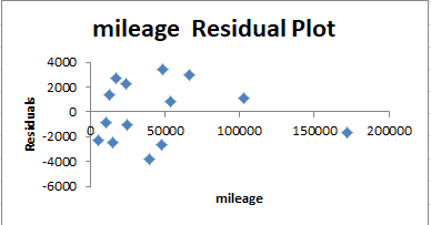
The above scatter plot indecates good fit