Question

Alternative Classification

How to Estimate Probabilities from Data? ( For continuous Attributes)

And How to generate an ensemble of classifiers?

Answer 1

aximum Likelihood Estimation (MLE)

Let P(H)=θ. θ, however, is unknown and all we have is D (sequence of heads and tails). So, what we can do to estimate θ is to choose its value such that the data is most likely.

MLE Principle: Find θ^ to maximize the likelihood of the data, P(D∣θ):

θ^MLE=argmaxθP(D∣θ)

For the sequence of coin flips we can use the binomial distribution to model P(D∣θ):

P(D∣θ)=(nH+nTnH)θnH(1−θ)nT

Now,

θ^MLE=argmaxθ(nH+nTnH)θnH(1−θ)nT=argmaxθlog(nH+nTnH)+nH⋅log(θ)+nT⋅log(1−θ)=argmaxθnH⋅log(θ)+nT⋅log(1−θ)

We can now solve for θ by taking the derivative and equating it to zero. This results in

nHθ=nT1−θ⟹nH−nHθ=nTθ⟹θ=nHnH+nT

Check: 1≥θ≥0 (no constraints necessary)

• MLE gives the explanation of the data you observed.
• If n

is large and your model/distribution is correct (that is H

• includes the true model), then MLE finds the true parameters.
• But the MLE can overfit the data if n
• is small. It works well when n
• is large.
• If you do not have the correct model (and n

• is small) then MLE can be terribly wrong!

For example, suppose you observe H,H,H,H,H. What is θ^MLE?

Simple scenario: coin toss with prior knowledge

Assume you have a hunch that θ is close to θ′=0.5. But your sample size is small, so you don't trust your estimate.

Simple fix: Add m imaginery throws that would result in θ′ (e.g. θ=0.5). Add m Heads and m Tails to your data.

θ^=nH+mnH+nT+2m

For large n, this is an insignificant change. For small n, it incorporates your "prior belief" about what θ should be.

Can we derive this formally?

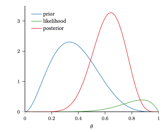
The Bayesian Way

Model θ as a random variable, drawn from a distribution P(θ). Note that θ is not a random variable associated with an event in a sample space. In frequentist statistics, this is forbidden. In Bayesian statistics, this is allowed.
Now, we can look at P(θ∣D)=P(D∣θ)P(θ)P(D) (recall Bayes Rule!), where

• P(D∣θ)

is the likelihood of the data given the parameter(s) θ

• ,
• P(θ)
• is the prior distribution over the parameter(s) θ
• , and
• P(θ∣D)
• is the posterior distribution over the parameter(s) θ
  • .
  
  
  Now, we can use the Beta distribution to model P(θ):

  P(θ)=θα−1(1−θ)β−1B(α,β)

  where B(α,β)=Γ(α)Γ(β)Γ(α+β) is the normalization constant. Note that here we only need a distribution over a binary random variable. The multivariate generalization of the Beta distribution is the Dirichlet distribution.
  
  Why using the Beta distribution?
  • it models probabilitis (θ
  lives on [0,1] and ∑iθi=1
• )
• it is of the same distributional family as the binomial distribution (conjugate prior) →

• the math will turn out nicely:

P(θ∣D)∝P(D∣θ)P(θ)∝θnH+α−1(1−θ)nT+β−1

Note taht in general θ are the parameters of our model. For the coin flipping scenario θ=P(H).
So far, we have a distribution over θ. How can we get an estimate for θ?

Maximum a Posteriori Probability Estimation (MAP)

For example, we can choose θ^ to be the most likely θ given the data.
MAP Principle: Find θ^ that maximizes the posterior distribution P(θ∣D):

θ^MAP=argmaxθP(θ∣D)=argmaxθlogP(D∣θ)+logP(θ)

For out coin flipping scenario, we get:

θ^MAP=argmaxθP(θ|Data)=argmaxθP(Data|θ)P(θ)P(Data)=argmaxθlog(P(Data|θ))+log(P(θ))=argmaxθnH⋅log(θ)+nT⋅log(1−θ)+(α−1)⋅log(θ)+(β−1)⋅log(1−θ)=argmaxθ(nH+α−1)⋅log(θ)+(nT+β−1)⋅log(1−θ)⟹θ^MAP=nH+α−1nH+nT+β+α−2(By Bayes rule)

• As n→∞

, θ^MAP→θ^MLE

• .
• MAP is a great estimator if prior belief exists and is accurate.
• If n

• is small, it can be very wrong if prior belief is wrong!

"True" Bayesian approach

Note that MAP is only one way to get an estimator for θ. There is much more information in P(θ∣D). So, instead of the maximum as we did with MAP, we can use the posterior mean (end even its variance).

θ^post_mean=E[θ,D]=∫θθP(θ∣D)dθ

For coin flipping, this can be computed as θ^post_mean=nH+αnH+α+nT+β.

Posterior Predictive Distribution

To make predictions using θ in our coin tossing example, we can use

P(heads∣D)=∫θP(heads,θ∣D)dθ=∫θP(heads∣θ,D)P(θ∣D)dθ=∫θθP(θ∣D)dθ

Here, we used the fact that we defined P(heads)=θ and that P(heads)=P(heads∣D,θ) (this is only the case for coin flipping - not in general).

In general, the posterior predictive distribution is

P(Y∣D,X)=∫θP(Y,θ∣D,X)dθ=∫θP(Y∣θ,D,X)P(θ|D)dθ

Unfortunately, the above is generally intractable in closed form and sampling techniques, such as Monte Carlo approximations, are used to approximate the distribution.

Machine Learning and estimation

In supervised Machine learning you are provided with training data D. You use this data to train a model, represented by its parameters θ. With this model you want to make predictions on a test point xt.

• MLE Prediction: P(y|xt;θ)

Learning: θ=argmaxθP(D;θ). Here θ