
Homework Answers
The regression model that is to be estimated is

where 
the estimated regression equation is

a) Using this
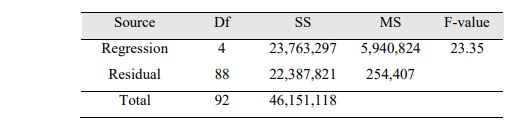
We know
k=4 is the number of independent variables
Sum of square Error (residuals), SSE = 22,387,821
degrees of freedom residuals = n-k-1 = 88
Sum of square Total (residuals), SST = 46,151,118
degrees of freedom total is n-1 = 92
The adjusted R-square is

ans: The adjusted R-square is 0.4929
b) We want to test the following hypotheses


The test statistics is F=23.35 with numerator df=4 and denominator df=88
Using F table for alpha=0.05 and numerator df=4 and denominator df=120 (The closest we can get to 88) we get the critical value of F = 2.45
We will reject the null hypothesis if the test statistics is greater than the critical value.
Here the test statistics is 23.35 and it is greater than the critical value, 2.45. Hence we reject the null hypothesis.
We conclude that the overall model is significant
c) There would be positive linear relationship between salary
and experience if the slope coefficient 
That is we want to test the following hypotheses

This is a right tailed test (the alternative hypothesis has ">").
The hypothesized value of 

Using the following
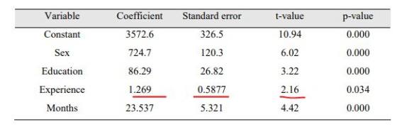
the test statistics is

The degrees of freedom for t statistics is n-k-1=88
The p-value given in the output is 0.034 is for a 2 tailed test. For one tailed test the p-value is half of that, that is p-value=0.034/2=0.017
We will reject the null hypothesis if the p-value is less than level of significance
Here the p-value is 0.017 and it is less than 0.05 level of significance. Hence we reject the null hypothesis.
We conclude that there is a positive linear relationship between Salary and Experience, after accounting for the effect of the variables, Sex, Education, and Months
d) the predicted salary for Sex=1 (man), Education = 15, Experience = 20 , months=10 is

ans: The salary for a man with 15 years of education, 20 months of experience and 10 months with in the company is $5,852.4
(Important: In the question pasted, the unit of the salary is not given. Please express the figure 5,852.4 accordingly)
e) To know if there is an interaction between Sex and Experience we will modify the model as below

If the interaction is significant it means that the coefficient

The salary model for a man is (by setting Sex=1)

The salary model for a woman (by setting sex=0) is

It means that the predicted salary changes by 

Add Answer to:
3. The table below shows the regression output of a multiple regression model relating the beginn...
Consider the following ANOVA table for a multiple regression model. Complete parts a through e be...
 *ANSWERS IN BOX ARE INCORRECT*
Consider the following ANOVA table for a multiple regression model. Complete parts a through e below. Source Regression 3 3,600 1200 20 Residual 35 2,100 60 Total df SSMSF 38 5,700 a. What is the size of this sample? n41 b. How many independent variables are in this model? c. Calculate the multiple coefficient of determination. R0.5882 Round to four decimal places as needed.) d. Test the significance of the overall regression model using α=0.05...
*ANSWERS IN BOX ARE INCORRECT*
Consider the following ANOVA table for a multiple regression model. Complete parts a through e below. Source Regression 3 3,600 1200 20 Residual 35 2,100 60 Total df SSMSF 38 5,700 a. What is the size of this sample? n41 b. How many independent variables are in this model? c. Calculate the multiple coefficient of determination. R0.5882 Round to four decimal places as needed.) d. Test the significance of the overall regression model using α=0.05...
The ANOVA summary table to the right is for a multiple regression model with five independent...
The ANOVA summary table to the right is for a multiple regression model with five independent variables. Complete parts (a) through (e). Source Degrees of Freedom Sum of Squares Regression 5 270 Error 28 110 Total 33 380 a. Determine the regression mean square (MSR) and the mean square error (MSE). b. Compute the overall FSTAT test statistic. FSTAT=_______________________ (Round to four decimal places as needed.) c. Determine whether there is a significant relationship between Y and the two independent...
. There is Stata output from a second OLS regression model with the variables defined as...
 . There is Stata output from a second OLS regression model with the variables defined as above. This time we include an interaction term "ageXgender" for the independent variables "age" and "gender." Use this output to answer parts g through i. regress casp age gender married agexgender df Number of obs- Source | 4,849 137.04 0.0000 0.1017 0.1009 6.0079 MS +FC4, 4844) 4,844 36.0944447 R-squared Model 19785.9491 4 4946.48728 Prob > F Residual 174841.49 Adj R-squared + Total 194627.439 4,848...
The tables below shows the results of a multiple linear regression analysis relating the sale price...
 The tables below shows the results of a multiple linear regression analysis relating the sale price y of a house (in dollars) versus LandVal (in dollars), Improvement (in dollars) and Area (in square feet): MS Source DF 877,967292656 46.66 100,349 6,272 978,316 0.00001 Regression 3 Residual16 Total 19 Predictor CoeffStd. ErrorT-valueP-value Intercept 1470 5746 0.26 0801 LandVal08145 0.5122 1.59 Improvement 0.8204 0.2112 3.88 2.05 0.131 0.001 Area 13.529 6.856 0.057 At alpha, a - 0.01 we can say that the...
Table 2 below shows cross-sectional regression results from the study of Beck, Degryse, and Kneer...
 Table 2 below shows cross-sectional regression results from the study of Beck, Degryse, and Kneer (2014).1 The dependent variable is the economic growth (GDP per capita growth) of different countries averaged over the period 1980- 2007. The explanatory variables are defined as follows: intermediation is a proxy for the size of financial sector and equal to the logarithm of the credit over GDP for every country in the sample; initial GDP is the logarithm of the GDP per capita in...
The ANOVA summary table to the right is for a multiple regression model with five independent variables. Complete parts (a) through (e). Source Degrees of Freedom Sum of Squares Regression 5 270 Err...
The ANOVA summary table to the right is for a multiple regression model with five independent variables. Complete parts (a) through (e). Source Degrees of Freedom Sum of Squares Regression 5 270 Error 28 110 Total 33 380 a. Determine the regression mean square (MSR) and the mean square error (MSE). b. Compute the overall FSTAT test statistic. FSTAT=_______________________ (Round to four decimal places as needed.) c. Determine whether there is a significant relationship between Y and the two independent...
Question 3 (3 points) The table below shows the regression results when calculating the least squares...
 Question 3 (3 points) The table below shows the regression results when calculating the least squares line of regression relating variable x (predictor) to variable y (response): Intercept Coefficients 0.083 1.417 Standard Error 3.56 0.63 t Star 0.02 2.25 P-value 0.9822 0.0745 Does variable x share a statistically significant linear relationship with variable y at the 5% significance level? Yes, since the p-value of 0.0745 is greater than 0.05. Yes, since the slope coefficient of 1.417 is less than the...
A real estate research firm has developed a regression model relating list price (Y in 1,000)...
 A real estate research firm has developed a regression model relating list price (Y in 1,000) with two independent variables. The two independent variables are number of bedrooms and size of the property. Part of the regression results are shown below. ANOVA MS Regression 256881.37 128440.68 Residual 42 726699.96 17302.38 Coefficients Standard Error Star Intercept 54.298 # Bedrooms 53.634 71.326 5.271 33.630 Acres 21.458 1. What has been the sample size? (2 Points) 2. What is the value of the...
SUMMARY OUTPUT Regression Statistics Multiple R 0.9655 R Square 0.9321 Adjusted R Square 0.9307 Standard Error...
 SUMMARY OUTPUT Regression Statistics Multiple R 0.9655 R Square 0.9321 Adjusted R Square 0.9307 Standard Error 0.5383 Observations 50 ANOVA df F 659.4383 Significance F 1.07386E-29 Regression Residual Total 1 48 49 SSM S 191.0842089 191.084209 13.90887066 0.28976814 204.9930796 Intercept Increase in profits (%) Coefficients Standard Error 2.28990 .0910 0.9513 0.0370 Stat 25.17540 25.6795 P-value .0000 0.0000 Lower 95% 2 .1070 0.8768 Upper 95% Lower 95.0%Jpper 95.0% 2.4728 2.1070 2.4728 1.0258 0.8768 10258 Increase in Manager's Salary (%) 4,00 2.00...
Question 4 3 pts Consider the estimated multiple regression model using OLS, with the standard errors...
 Question 4 3 pts Consider the estimated multiple regression model using OLS, with the standard errors in parentheses below each estimated coefficient. There are 1,576 observations in the sample: Y = 10 + 2X2i - 5Xzi (3) (1.5) (2) Suppose that the sample mean of Y is 30. For the 18th observation (i=18) in the sample, the value of X2 is 50, the value of X3 is 16, and the value of Y is 20. The residual associated with the...
 *ANSWERS IN BOX ARE INCORRECT*
Consider the following ANOVA table for a multiple regression model. Complete parts a through e below. Source Regression 3 3,600 1200 20 Residual 35 2,100 60 Total df SSMSF 38 5,700 a. What is the size of this sample? n41 b. How many independent variables are in this model? c. Calculate the multiple coefficient of determination. R0.5882 Round to four decimal places as needed.) d. Test the significance of the overall regression model using α=0.05...
*ANSWERS IN BOX ARE INCORRECT*
Consider the following ANOVA table for a multiple regression model. Complete parts a through e below. Source Regression 3 3,600 1200 20 Residual 35 2,100 60 Total df SSMSF 38 5,700 a. What is the size of this sample? n41 b. How many independent variables are in this model? c. Calculate the multiple coefficient of determination. R0.5882 Round to four decimal places as needed.) d. Test the significance of the overall regression model using α=0.05...
 . There is Stata output from a second OLS regression model with the variables defined as above. This time we include an interaction term "ageXgender" for the independent variables "age" and "gender." Use this output to answer parts g through i. regress casp age gender married agexgender df Number of obs- Source | 4,849 137.04 0.0000 0.1017 0.1009 6.0079 MS +FC4, 4844) 4,844 36.0944447 R-squared Model 19785.9491 4 4946.48728 Prob > F Residual 174841.49 Adj R-squared + Total 194627.439 4,848...
 The tables below shows the results of a multiple linear regression analysis relating the sale price y of a house (in dollars) versus LandVal (in dollars), Improvement (in dollars) and Area (in square feet): MS Source DF 877,967292656 46.66 100,349 6,272 978,316 0.00001 Regression 3 Residual16 Total 19 Predictor CoeffStd. ErrorT-valueP-value Intercept 1470 5746 0.26 0801 LandVal08145 0.5122 1.59 Improvement 0.8204 0.2112 3.88 2.05 0.131 0.001 Area 13.529 6.856 0.057 At alpha, a - 0.01 we can say that the...
 Table 2 below shows cross-sectional regression results from the study of Beck, Degryse, and Kneer (2014).1 The dependent variable is the economic growth (GDP per capita growth) of different countries averaged over the period 1980- 2007. The explanatory variables are defined as follows: intermediation is a proxy for the size of financial sector and equal to the logarithm of the credit over GDP for every country in the sample; initial GDP is the logarithm of the GDP per capita in...
 Question 3 (3 points) The table below shows the regression results when calculating the least squares line of regression relating variable x (predictor) to variable y (response): Intercept Coefficients 0.083 1.417 Standard Error 3.56 0.63 t Star 0.02 2.25 P-value 0.9822 0.0745 Does variable x share a statistically significant linear relationship with variable y at the 5% significance level? Yes, since the p-value of 0.0745 is greater than 0.05. Yes, since the slope coefficient of 1.417 is less than the...
 A real estate research firm has developed a regression model relating list price (Y in 1,000) with two independent variables. The two independent variables are number of bedrooms and size of the property. Part of the regression results are shown below. ANOVA MS Regression 256881.37 128440.68 Residual 42 726699.96 17302.38 Coefficients Standard Error Star Intercept 54.298 # Bedrooms 53.634 71.326 5.271 33.630 Acres 21.458 1. What has been the sample size? (2 Points) 2. What is the value of the...
 SUMMARY OUTPUT Regression Statistics Multiple R 0.9655 R Square 0.9321 Adjusted R Square 0.9307 Standard Error 0.5383 Observations 50 ANOVA df F 659.4383 Significance F 1.07386E-29 Regression Residual Total 1 48 49 SSM S 191.0842089 191.084209 13.90887066 0.28976814 204.9930796 Intercept Increase in profits (%) Coefficients Standard Error 2.28990 .0910 0.9513 0.0370 Stat 25.17540 25.6795 P-value .0000 0.0000 Lower 95% 2 .1070 0.8768 Upper 95% Lower 95.0%Jpper 95.0% 2.4728 2.1070 2.4728 1.0258 0.8768 10258 Increase in Manager's Salary (%) 4,00 2.00...
 Question 4 3 pts Consider the estimated multiple regression model using OLS, with the standard errors in parentheses below each estimated coefficient. There are 1,576 observations in the sample: Y = 10 + 2X2i - 5Xzi (3) (1.5) (2) Suppose that the sample mean of Y is 30. For the 18th observation (i=18) in the sample, the value of X2 is 50, the value of X3 is 16, and the value of Y is 20. The residual associated with the...
Most questions answered within 3 hours.
-
Where is the error in this code sequence?
String s1 = "Hello";
String s2 = "ello";...
asked 11 months ago -
Financial data for Joel de Paris, Inc., for last year
follow:
Joel de Paris, Inc.
Balance...
asked 11 months ago -
Consider this reaction:
Al2(SO4)3 (aq)+ BaCl3
(aq) Al2Cl6 (aq)- +
3BaSO4(s) . What is the...
asked 11 months ago -
Suppose that Savneet is considering increasing her
recent random sample from 20 car rentals to 40...
asked 11 months ago -
Trucks arrive at an unloading terminal at an average rate of 120
per hour.
Trucks arrive...
asked 11 months ago -
Why are methanol and ethanol completely soluble in water while
octanol is not very little soluble....
asked 11 months ago -
A facilities manager at a university reads in a research report
that the mean amount of...
asked 11 months ago -
When the CuSO4 is rehydrated by adding water to the anhydrous
compound, is this an endothermic...
asked 11 months ago -
A ray of sunlight is passing from diamond into crown glass; the
angle of incidence is...
asked 11 months ago -
A block of mass 0.249 kg is placed on top of a light, vertical
spring of...
asked 11 months ago -
how do the kidneys compensate in the presences of acidosis
a) trigger hyperventilate
b) reserve acid...
asked 11 months ago -
Question 501 pts
The rental rate of capital to the firm increases. Which of the
following...
asked 11 months ago