0 0 0.1 0.2 0.3 0.4 0.5 0.6 0 0.1 0.2 0.3 0.4 0.5 0.6 0.1 0.2 0.3 0.4 0.5 0.6 0 0 0.1 0.2 0.3 0.4 0.5 0.6
Homework Answers

Add Answer to:
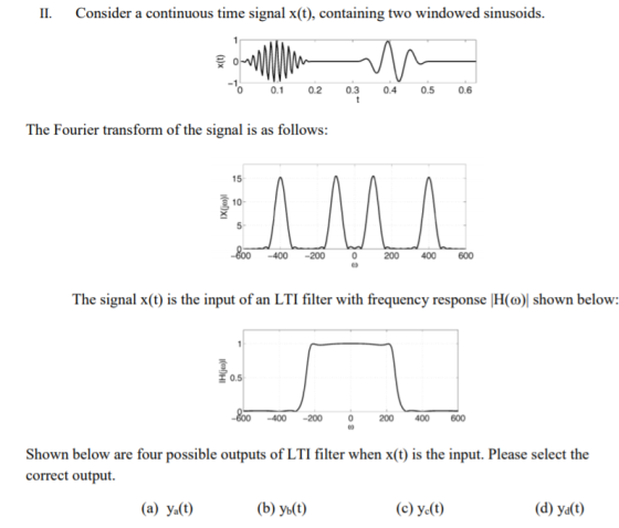
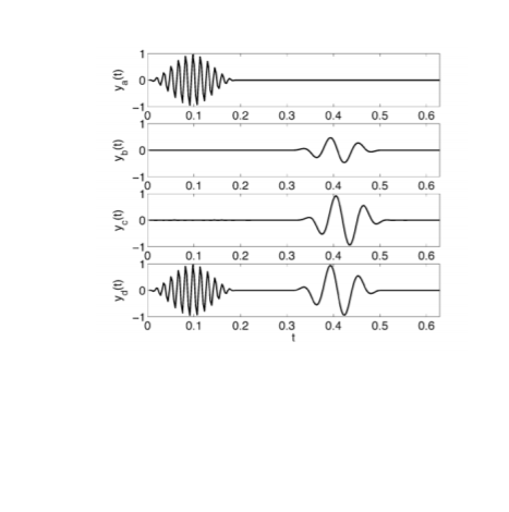
II. Consider a continuous time signal x(t), containing two windowed sinusoids 0.1 0.2 0.3 0.4 0.5...
Create chart or table Consider the system with the impulse response ht)e u(t), as shown in Figure...
 Create chart or table Consider the system with the impulse response ht)e u(t), as shown in Figure 3.2(a). This system's response to an input of x(t) 1) would be y(t) h(r ult 1). as shown in Figure 3.2(b). If the input signal is a sum of weighted, time-shifted impulses as described by (3.10), separated in time by Δ = 0.1 (s) so that xt)01-0.1k), as shown in Figure 3.2(c), then, according to (3.11), the output is This output signal is...
6. The distribution law of random variable X is given -0.4 |-0.2 |0 0.1 0.4 0.3...
 6. The distribution law of random variable X is given -0.4 |-0.2 |0 0.1 0.4 0.3 0 0.6 0.2 Pi Find the variance of random variable X. nrohahility density function is:
H (calories/m3) 600 500 400 300 H(T,0.4) Н (Т, 0.3) 200 Н(T, 0.2) 100 Н(Т,0.1) T...
 H (calories/m3) 600 500 400 300 H(T,0.4) Н (Т, 0.3) 200 Н(T, 0.2) 100 Н(Т,0.1) T (oC) 40 0 10 20 n 30 Figure 14.17 31. Use Figure 14.17 to estimate HT (10,0.1). Interpret the partial derivative in practical terms. 1 A 17
H (calories/m3) 600 500 400 300 H(T,0.4) Н (Т, 0.3) 200 Н(T, 0.2) 100 Н(Т,0.1) T (oC) 40 0 10 20 n 30 Figure 14.17 31. Use Figure 14.17 to estimate HT (10,0.1). Interpret the partial derivative...
H (calories/m3) 600 500 400 300 H(T,0.4) Н (Т, 0.3) 200 Н(T, 0.2) 100 Н(Т,0.1) T (oC) 40 0 10 20 n 30 Figure 14.17 31. Use Figure 14.17 to estimate HT (10,0.1). Interpret the partial derivative in practical terms. 1 A 17
H (calories/m3) 600 500 400 300 H(T,0.4) Н (Т, 0.3) 200 Н(T, 0.2) 100 Н(Т,0.1) T (oC) 40 0 10 20 n 30 Figure 14.17 31. Use Figure 14.17 to estimate HT (10,0.1). Interpret the partial derivative...
3. The system represented by the block diagram below modulates the message signal x(t) with a carrier wave c(t) to yield -(). The signal y(t) is generated by multiplying z() by the carrier wave c(t)....
 3. The system represented by the block diagram below modulates the message signal x(t) with a carrier wave c(t) to yield -(). The signal y(t) is generated by multiplying z() by the carrier wave c(t). c(t) c(t) y(t) z(t) The output signal,y(t), can be written as y(t)-C() × X() x C(t). Using the properties of a) Fourier Transforms, write Yi) in terms of Cjo) and Yj). [2 points] The Fourier Transform of x(t) is illustrated below. 0.9 0.8 0.7 0.6...
6. The distribution law of random variable X is given -0.4 -0.2 0 0.1 0.4 0.3...
 6. The distribution law of random variable X is given -0.4 -0.2 0 0.1 0.4 0.3 0.2 0.6 Xi Pi Find the variance of random variable X. 7. Let X be a continuous random variable whose probability density function is: f(x)=Ice + ax, ifXE (0,1) if x ¢ (0:1) 0, Find 1) the coefficient a; 2) P(O.5 X<0.7); 3) P(X>3). Part 3. Statistics A sample of measurements is given Y 8 4 2 2 0 8. Compute the coefficient of...
Don't need to do #1. Please go into detail on how you solved #2 and #3 The Fourier transform of the signal r(t) is given by the following figure (X(jw)0 for w> 20) X(ju) 0.8 0.6 0.4 0.2 -10 10...
 Don't need to do #1. Please go into detail on how you solved #2
and #3
The Fourier transform of the signal r(t) is given by the following figure (X(jw)0 for w> 20) X(ju) 0.8 0.6 0.4 0.2 -10 10 20 m Page 4 of 5 Final S09 EE315 Signals & Systems The signal is sampled to obtain the signal withFourier transform Xlw 1. (5p) What is the minimum sampling frequency w 2. (10p) Now suppose that the sampling frequency...
Don't need to do #1. Please go into detail on how you solved #2
and #3
The Fourier transform of the signal r(t) is given by the following figure (X(jw)0 for w> 20) X(ju) 0.8 0.6 0.4 0.2 -10 10 20 m Page 4 of 5 Final S09 EE315 Signals & Systems The signal is sampled to obtain the signal withFourier transform Xlw 1. (5p) What is the minimum sampling frequency w 2. (10p) Now suppose that the sampling frequency...
Q. 2 A continuous time signal x(t) has the Continuous Time Fourier Transform shown in Fig...
 Q. 2 A continuous time signal x(t) has the Continuous Time Fourier Transform shown in Fig 2. Xc() -80007 0 80001 2 (rad/s) Fig 2 According to the sampling theorem, find the maximum allowable sampling period T for this signal. Also plot the Fourier Transforms of the sampled signal X:(j) and X(elo). Label the resulting signals appropriately (both in frequency and amplitude axis). Assuming that the sampling period is increased 1.2 times, what is the new sampling frequency 2? What...
4. Using Matlab: 4.1. Plot | H(n the following cases: (the frequency range: 0-20 KHz) a. a 0.2 0.5 ms. b. α-0.8 C.α-0.2 c-0.1 ms. c 0.5 ms. 4.2. Consider a signal whose Fourier Transform is given...
 4. Using Matlab: 4.1. Plot | H(n the following cases: (the frequency range: 0-20 KHz) a. a 0.2 0.5 ms. b. α-0.8 C.α-0.2 c-0.1 ms. c 0.5 ms. 4.2. Consider a signal whose Fourier Transform is given by: 50000ω Plot the transfer function l x(o) l and the output l Y(o) l in each of the above cases (stated in part 4.1) 4.3. Find the Inverse Fourier Transorms of| X(oand Y(o) , and generate the audio signals x and y...
Consider the following probability distribution: x P(x) 1 0.1 2 ? 3 0.2 4 0.3 What...
Consider the following probability distribution: x P(x) 1 0.1 2 ? 3 0.2 4 0.3 What must be the value of P(2) if the distribution is valid? A. 0.6 B. 0.5 C. 0.4 D. 0.2 What is the mean of the probability distribution? A. 2.5 B. 2.7 C. 2.0 D. 2.9
Consider the probability distribution shown below: X 10 12 18 20 p(x) 0.2 0.3 0.1 0.4...
Consider the probability distribution shown below: X 10 12 18 20 p(x) 0.2 0.3 0.1 0.4 Find the standard deviation of X.
 Create chart or table Consider the system with the impulse response ht)e u(t), as shown in Figure 3.2(a). This system's response to an input of x(t) 1) would be y(t) h(r ult 1). as shown in Figure 3.2(b). If the input signal is a sum of weighted, time-shifted impulses as described by (3.10), separated in time by Δ = 0.1 (s) so that xt)01-0.1k), as shown in Figure 3.2(c), then, according to (3.11), the output is This output signal is...
 6. The distribution law of random variable X is given -0.4 |-0.2 |0 0.1 0.4 0.3 0 0.6 0.2 Pi Find the variance of random variable X. nrohahility density function is:
 H (calories/m3) 600 500 400 300 H(T,0.4) Н (Т, 0.3) 200 Н(T, 0.2) 100 Н(Т,0.1) T (oC) 40 0 10 20 n 30 Figure 14.17 31. Use Figure 14.17 to estimate HT (10,0.1). Interpret the partial derivative in practical terms. 1 A 17
H (calories/m3) 600 500 400 300 H(T,0.4) Н (Т, 0.3) 200 Н(T, 0.2) 100 Н(Т,0.1) T (oC) 40 0 10 20 n 30 Figure 14.17 31. Use Figure 14.17 to estimate HT (10,0.1). Interpret the partial derivative...
H (calories/m3) 600 500 400 300 H(T,0.4) Н (Т, 0.3) 200 Н(T, 0.2) 100 Н(Т,0.1) T (oC) 40 0 10 20 n 30 Figure 14.17 31. Use Figure 14.17 to estimate HT (10,0.1). Interpret the partial derivative in practical terms. 1 A 17
H (calories/m3) 600 500 400 300 H(T,0.4) Н (Т, 0.3) 200 Н(T, 0.2) 100 Н(Т,0.1) T (oC) 40 0 10 20 n 30 Figure 14.17 31. Use Figure 14.17 to estimate HT (10,0.1). Interpret the partial derivative...
 3. The system represented by the block diagram below modulates the message signal x(t) with a carrier wave c(t) to yield -(). The signal y(t) is generated by multiplying z() by the carrier wave c(t). c(t) c(t) y(t) z(t) The output signal,y(t), can be written as y(t)-C() × X() x C(t). Using the properties of a) Fourier Transforms, write Yi) in terms of Cjo) and Yj). [2 points] The Fourier Transform of x(t) is illustrated below. 0.9 0.8 0.7 0.6...
 6. The distribution law of random variable X is given -0.4 -0.2 0 0.1 0.4 0.3 0.2 0.6 Xi Pi Find the variance of random variable X. 7. Let X be a continuous random variable whose probability density function is: f(x)=Ice + ax, ifXE (0,1) if x ¢ (0:1) 0, Find 1) the coefficient a; 2) P(O.5 X<0.7); 3) P(X>3). Part 3. Statistics A sample of measurements is given Y 8 4 2 2 0 8. Compute the coefficient of...
 Don't need to do #1. Please go into detail on how you solved #2
and #3
The Fourier transform of the signal r(t) is given by the following figure (X(jw)0 for w> 20) X(ju) 0.8 0.6 0.4 0.2 -10 10 20 m Page 4 of 5 Final S09 EE315 Signals & Systems The signal is sampled to obtain the signal withFourier transform Xlw 1. (5p) What is the minimum sampling frequency w 2. (10p) Now suppose that the sampling frequency...
Don't need to do #1. Please go into detail on how you solved #2
and #3
The Fourier transform of the signal r(t) is given by the following figure (X(jw)0 for w> 20) X(ju) 0.8 0.6 0.4 0.2 -10 10 20 m Page 4 of 5 Final S09 EE315 Signals & Systems The signal is sampled to obtain the signal withFourier transform Xlw 1. (5p) What is the minimum sampling frequency w 2. (10p) Now suppose that the sampling frequency...
 Q. 2 A continuous time signal x(t) has the Continuous Time Fourier Transform shown in Fig 2. Xc() -80007 0 80001 2 (rad/s) Fig 2 According to the sampling theorem, find the maximum allowable sampling period T for this signal. Also plot the Fourier Transforms of the sampled signal X:(j) and X(elo). Label the resulting signals appropriately (both in frequency and amplitude axis). Assuming that the sampling period is increased 1.2 times, what is the new sampling frequency 2? What...
 4. Using Matlab: 4.1. Plot | H(n the following cases: (the frequency range: 0-20 KHz) a. a 0.2 0.5 ms. b. α-0.8 C.α-0.2 c-0.1 ms. c 0.5 ms. 4.2. Consider a signal whose Fourier Transform is given by: 50000ω Plot the transfer function l x(o) l and the output l Y(o) l in each of the above cases (stated in part 4.1) 4.3. Find the Inverse Fourier Transorms of| X(oand Y(o) , and generate the audio signals x and y...
Most questions answered within 3 hours.
-
Where is the error in this code sequence?
String s1 = "Hello";
String s2 = "ello";...
asked 11 months ago -
Financial data for Joel de Paris, Inc., for last year
follow:
Joel de Paris, Inc.
Balance...
asked 11 months ago -
Consider this reaction:
Al2(SO4)3 (aq)+ BaCl3
(aq) Al2Cl6 (aq)- +
3BaSO4(s) . What is the...
asked 11 months ago -
Suppose that Savneet is considering increasing her
recent random sample from 20 car rentals to 40...
asked 11 months ago -
Trucks arrive at an unloading terminal at an average rate of 120
per hour.
Trucks arrive...
asked 11 months ago -
Why are methanol and ethanol completely soluble in water while
octanol is not very little soluble....
asked 11 months ago -
A facilities manager at a university reads in a research report
that the mean amount of...
asked 11 months ago -
When the CuSO4 is rehydrated by adding water to the anhydrous
compound, is this an endothermic...
asked 11 months ago -
A ray of sunlight is passing from diamond into crown glass; the
angle of incidence is...
asked 11 months ago -
A block of mass 0.249 kg is placed on top of a light, vertical
spring of...
asked 11 months ago -
how do the kidneys compensate in the presences of acidosis
a) trigger hyperventilate
b) reserve acid...
asked 11 months ago -
Question 501 pts
The rental rate of capital to the firm increases. Which of the
following...
asked 11 months ago