Only question 6 please, this is the model referred to in
Question 6 from 5.c
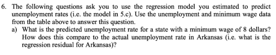

6. The following questions ask you to use the regression model you estimated to predict unemployment rates (ie, the model in 5.c). Use the unemployment and minimum wage data from the table above to answer this question. a) What is the predicted unemployment rate for a state with a minimum wage of 8 dollars? How does this compare to the actual unemployment rate in Arkansas (i.e. what is the regression residual for Arkansas)?
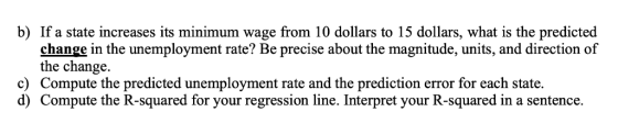
b) If a state increases its minimum wage from 10 dollars to 15 dollars, what is the predicted change in the unemployment rate? Be precise about the magnitude, units, and direction of the change. c) Compute the predicted unemployment rate and the prediction error for each state. d) Compute the R-squared for your regression line. Interpret your R-squared in a sentence.
State 2018 Minimum Rate (%) Wage $7 $11 $8 Unemployment Alabama Arizona Arkansas California$11 DC 4 4 6 $13
Homework Answers
6.
Sol:
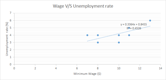
Unemployment rate = 0.3364*wage + 0.8455
A.
For a minimum wage of $10.
Predicted unemployment rate = 0.3364*10 + 0.8455
Predicted unemployment rate = 4.21%
Actual unemployment rate in Colorado = 3%
So, predicted unemployment rate in Colorado is overstated by 1.21%
B.
For a minimum wage of $15.
Predicted unemployment rate = 0.3364*15 + 0.8455 = 5.89%
Change in predicted unemployment rate = 5.89%-4.21% = 1.68%
C.
| State | 2018 Minimum wage ($) | Unemployment rate % | Predicted unemployment rate (%) | Prediction error |
| Alabama | 7 | 4 | 3.20 | 0.80 |
| Arizona | 11 | 5 | 4.55 | 0.45 |
| Arkansas | 8 | 3 | 3.54 | -0.54 |
| California | 11 | 4 | 4.55 | -0.55 |
| DC | 13 | 6 | 5.22 | 0.78 |
D.
R Square = 45.26%
The minimum wage can only explain 45.26% of the change in unemployment rate.
Add Answer to:
C) Estimate the linear model for a state's unemployment rate shown below (i.e. estimate Bo and β1...
5. Use the unemployment and minimum wage data above to answer this question. a) What is...
 5. Use the unemployment and minimum wage data above to answer this question. a) What is the predicted unemployment rate for a state with a minimum wage of 10 dollars? How does this compare to the actual unemployment rate in Colorado? If a state increases its minimum wage from 10 dollars to 15 dollars, what is the predicted change in the unemployment rate? b) c) Compute the predicted unemployment rate and the prediction error for each state. d) Compute the...
ys 70 eoni idence interval for μο 4. The following table contains the minimum wage and...
 ys 70 eoni idence interval for μο 4. The following table contains the minimum wage and unemployment rates for a sample of eight states. State 2018 Unemployment | Minimum | Rate (96) Wage Alabama Arizona Arkansas S7 $11 $8 California $11 4 Colorado $10 Connecticut $10 $8 $13 Delaware DC 4 Graph unemployment and minimum wage, with unemployment on the vertical axis. Draw a line that best fits the points and label the intercept and slope. You can use your...
The homeownership rate in the US. was 61.4% in 2009, In order to determine if homeownership is li...
 The homeownership rate in the US. was 61.4% in 2009, In order to determine if homeownership is linked with income, 2009 state-level data on the homeownership rate (Ownership in %) and median household income (income in $) were collected. A portion of the data is shown in the accompanying table State Alabama Alaska ownership Income 36,000 57,624 66.7 62.5 Wyoming 68.2 48,490 XC a-1. Estimate the model Ownership = β0 + β1Income + ε. (Negative values should be indicated by...
Suppose you estimate the following model by OLS: wage = β0 + β1educ + β2exper +...
Suppose you estimate the following model by OLS: wage = β0 + β1educ + β2exper + u wage : hourly age in dollars educ : years of education exper : years of experience You obtain the following fitted model using STATA, where standard errors are given in parenthesis wage [ = 3.5 + 0.9educ + 1.5exper (2.0) (0.7) (0.5) Number obs. : 523 R 2 = 0.45 For the following questions, make use to the relevant statistical tables. If you...
QUESTION 1 Consider the following OLS regression line (or sample regression function): wage =-2.10+ 0.50 educ...
 QUESTION 1 Consider the following OLS regression line (or sample regression function): wage =-2.10+ 0.50 educ (1), where wage is hourly wage, measured in dollars, and educ years of formal education. According to (1), a person with no education has a predicted hourly wage of [wagehat] dollars. (NOTE: Write your answer in number format, with 2 decimal places of precision level; do not write your answer as a fraction. Add a leading minus sign symbol, a leading zero and trailing...
12. Which coefficient(s) is (are) significant at the .05 level? Select one: a. Income, Unemployment and...
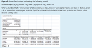 12. Which
coefficient(s) is (are) significant at the .05
level?
Select one:
a. Income, Unemployment and Pupil/Tea
b. Divorce
c. Income and Pupil/Tea
d. Income
PART B-- Refer to Figure 2
Is the regression equation significant at the .05
level?
Select one:
a. YES
b. NO
c. Need more information to answer this question
PART C-- Refer to Figure 2
Which of the following is a correct interpretation for
the variable Unem?
Select one:
a. Unemployed people steal 40.63 more...
12. Which
coefficient(s) is (are) significant at the .05
level?
Select one:
a. Income, Unemployment and Pupil/Tea
b. Divorce
c. Income and Pupil/Tea
d. Income
PART B-- Refer to Figure 2
Is the regression equation significant at the .05
level?
Select one:
a. YES
b. NO
c. Need more information to answer this question
PART C-- Refer to Figure 2
Which of the following is a correct interpretation for
the variable Unem?
Select one:
a. Unemployed people steal 40.63 more...
Consider a multiple linear regression model Y; = Bo + B1Xi1 + B22:2 + 33213 +...
 Consider a multiple linear regression model Y; = Bo + B1Xi1 + B22:2 + 33213 + Blog(x14) + Ej. We have the following statistics for the regression Call: 1m formula = y “ x1 + x2 + x3 + log(x4) Coefficients: Estimate Std. Error t value Pr(>1t|) (Intercept) 154.1928 194.9062 0.791 0.432938 x1 -4.2280 2.0301 -2.083 0.042873 * x2 -6.1353 2.1936 -2.797 0.007508 ** x3 0.4719 0.1285 3.672 0.000626 *** x4 26.7552 9.3374 2.865 0.006259 ** Signif. codes: O '***'...
Consider a multiple linear regression model Y; = Bo + B1Xi1 + B22:2 + 33213 +...
 Consider a multiple linear regression model Y; = Bo + B1Xi1 + B22:2 + 33213 + Blog(x14) + Ej. We have the following statistics for the regression Call: 1m formula = y “ x1 + x2 + x3 + log(x4) Coefficients: Estimate Std. Error t value Pr(>1t|) (Intercept) 154.1928 194.9062 0.791 0.432938 x1 -4.2280 2.0301 -2.083 0.042873 * x2 -6.1353 2.1936 -2.797 0.007508 ** x3 0.4719 0.1285 3.672 0.000626 *** x4 26.7552 9.3374 2.865 0.006259 ** Signif. codes: O '***'...
2. Use the data in hpricel.wfl uploaded on Moodle for this exercise. We assume that all assump- tions of the Classical Linear Model are satisfied for the model used in this question....
 2. Use the data in hpricel.wfl uploaded on Moodle for this exercise. We assume that all assump- tions of the Classical Linear Model are satisfied for the model used in this question. (a) Estimate the model and report the results in the usual form, including the standard error of the regression. Obtain the predicted price when we plug in lotsize - 10, 000, sqrft - 2,300, and bdrms- 4; round this price to the nearest dollar. (b) Run a regression...
 5. Use the unemployment and minimum wage data above to answer this question. a) What is the predicted unemployment rate for a state with a minimum wage of 10 dollars? How does this compare to the actual unemployment rate in Colorado? If a state increases its minimum wage from 10 dollars to 15 dollars, what is the predicted change in the unemployment rate? b) c) Compute the predicted unemployment rate and the prediction error for each state. d) Compute the...
 ys 70 eoni idence interval for μο 4. The following table contains the minimum wage and unemployment rates for a sample of eight states. State 2018 Unemployment | Minimum | Rate (96) Wage Alabama Arizona Arkansas S7 $11 $8 California $11 4 Colorado $10 Connecticut $10 $8 $13 Delaware DC 4 Graph unemployment and minimum wage, with unemployment on the vertical axis. Draw a line that best fits the points and label the intercept and slope. You can use your...
 The homeownership rate in the US. was 61.4% in 2009, In order to determine if homeownership is linked with income, 2009 state-level data on the homeownership rate (Ownership in %) and median household income (income in $) were collected. A portion of the data is shown in the accompanying table State Alabama Alaska ownership Income 36,000 57,624 66.7 62.5 Wyoming 68.2 48,490 XC a-1. Estimate the model Ownership = β0 + β1Income + ε. (Negative values should be indicated by...
 QUESTION 1 Consider the following OLS regression line (or sample regression function): wage =-2.10+ 0.50 educ (1), where wage is hourly wage, measured in dollars, and educ years of formal education. According to (1), a person with no education has a predicted hourly wage of [wagehat] dollars. (NOTE: Write your answer in number format, with 2 decimal places of precision level; do not write your answer as a fraction. Add a leading minus sign symbol, a leading zero and trailing...
 12. Which
coefficient(s) is (are) significant at the .05
level?
Select one:
a. Income, Unemployment and Pupil/Tea
b. Divorce
c. Income and Pupil/Tea
d. Income
PART B-- Refer to Figure 2
Is the regression equation significant at the .05
level?
Select one:
a. YES
b. NO
c. Need more information to answer this question
PART C-- Refer to Figure 2
Which of the following is a correct interpretation for
the variable Unem?
Select one:
a. Unemployed people steal 40.63 more...
12. Which
coefficient(s) is (are) significant at the .05
level?
Select one:
a. Income, Unemployment and Pupil/Tea
b. Divorce
c. Income and Pupil/Tea
d. Income
PART B-- Refer to Figure 2
Is the regression equation significant at the .05
level?
Select one:
a. YES
b. NO
c. Need more information to answer this question
PART C-- Refer to Figure 2
Which of the following is a correct interpretation for
the variable Unem?
Select one:
a. Unemployed people steal 40.63 more...
 Consider a multiple linear regression model Y; = Bo + B1Xi1 + B22:2 + 33213 + Blog(x14) + Ej. We have the following statistics for the regression Call: 1m formula = y “ x1 + x2 + x3 + log(x4) Coefficients: Estimate Std. Error t value Pr(>1t|) (Intercept) 154.1928 194.9062 0.791 0.432938 x1 -4.2280 2.0301 -2.083 0.042873 * x2 -6.1353 2.1936 -2.797 0.007508 ** x3 0.4719 0.1285 3.672 0.000626 *** x4 26.7552 9.3374 2.865 0.006259 ** Signif. codes: O '***'...
 Consider a multiple linear regression model Y; = Bo + B1Xi1 + B22:2 + 33213 + Blog(x14) + Ej. We have the following statistics for the regression Call: 1m formula = y “ x1 + x2 + x3 + log(x4) Coefficients: Estimate Std. Error t value Pr(>1t|) (Intercept) 154.1928 194.9062 0.791 0.432938 x1 -4.2280 2.0301 -2.083 0.042873 * x2 -6.1353 2.1936 -2.797 0.007508 ** x3 0.4719 0.1285 3.672 0.000626 *** x4 26.7552 9.3374 2.865 0.006259 ** Signif. codes: O '***'...
 2. Use the data in hpricel.wfl uploaded on Moodle for this exercise. We assume that all assump- tions of the Classical Linear Model are satisfied for the model used in this question. (a) Estimate the model and report the results in the usual form, including the standard error of the regression. Obtain the predicted price when we plug in lotsize - 10, 000, sqrft - 2,300, and bdrms- 4; round this price to the nearest dollar. (b) Run a regression...
Most questions answered within 3 hours.
-
Where is the error in this code sequence?
String s1 = "Hello";
String s2 = "ello";...
asked 11 months ago -
Financial data for Joel de Paris, Inc., for last year
follow:
Joel de Paris, Inc.
Balance...
asked 11 months ago -
Consider this reaction:
Al2(SO4)3 (aq)+ BaCl3
(aq) Al2Cl6 (aq)- +
3BaSO4(s) . What is the...
asked 11 months ago -
Suppose that Savneet is considering increasing her
recent random sample from 20 car rentals to 40...
asked 11 months ago -
Trucks arrive at an unloading terminal at an average rate of 120
per hour.
Trucks arrive...
asked 11 months ago -
Why are methanol and ethanol completely soluble in water while
octanol is not very little soluble....
asked 11 months ago -
A facilities manager at a university reads in a research report
that the mean amount of...
asked 11 months ago -
When the CuSO4 is rehydrated by adding water to the anhydrous
compound, is this an endothermic...
asked 11 months ago -
A ray of sunlight is passing from diamond into crown glass; the
angle of incidence is...
asked 11 months ago -
A block of mass 0.249 kg is placed on top of a light, vertical
spring of...
asked 11 months ago -
how do the kidneys compensate in the presences of acidosis
a) trigger hyperventilate
b) reserve acid...
asked 11 months ago -
Question 501 pts
The rental rate of capital to the firm increases. Which of the
following...
asked 11 months ago