Question

Capacity List Price Maytag High-Efficiency Top Loading Washer with Steanm Samsung High-Efficiency Top Loading Washer with Active 4.8 $749 Wash and Integrated Touch Controls Whirlpool High-Efficiency Front Loading Washer with Steam Maytag High-Efficiency Top Loading Washer Whirlpool High-Efficiency Top Loading Washer Samsung High-Efficiency Froat Loading Washer Samsung High Efficiency Front Loading Washer with 5.0 $1,299 4.3 4.3 AddWash Door 4.5 Whirlpool High-Efficiency Front Loading Washer 4.5 Whirlpool High Efficiency Top Loading Washer with Stearm Samsung High-Efficiency Top Loading Washer with ActiveWash Whirlpool High Efficiency Top Loading Washer Maytag High-Efficiency Front Loading Washer with Steam Whirlpool High-Efficiency Front Loading Washer with Steam Maytag High-Efficiency Top Loading Washer Samsung High-Efficiency Top Loading Washer Maytag High-Efficiency Front Loading Washer with Steam Samsung High-Efliciency Top Loading Washer with 4.8 4.8 4.3 4.5 5.3 4.8 4.5 $899 $1,099 ActiveWash and Integrated Touch Controls Samsung High-Efliciency Top Loading Washer Samsung High-Efliciency Front Loading Washer with Steam Whirlpool High-Efficiency Front Loading Washer with Steam Whirlpool High Elliciency Front Loading Washer Samsung High-Efficiency Top Loading Washer with 4.5 4.5 5.6 4.5 4.2 $1,599 $1,099 5.2 5,3 5.3 $1.199 $1,099 $1.199 Maytag High-Efficiency Top Loading Washer with Steam Whirlpool High-Efficiency Top Loading Washer with Steam 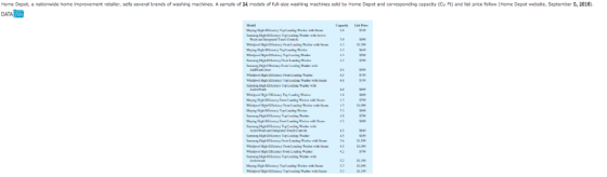Home Depot, a nationwide home improvement retailer, sells several brands of washing machines. A sample of 24 models of full-size washing machines sold by Home Depot and corresponding capacity (Cu Ft) and list price follow (Home Depot website, September 5, 2016) DATA a. Which of the following scatter diagrams are represent the data, treating cubic feet as the independent variable. A LsPrice 5) Capacity B Price Capacty Price5) Capacity -Select your answer- Does a simple linear regression model appear to be appropriate? -Select your answer - b. Use a simple regression model to develop an estimated regression equation to predict the list price given the cubic feet (to 4 decimals). Enter negative value as negative number. Capacity + 8. Select your answer- Based upon the standardized residual plot, does a simple linear regression model appear to be appropriate? -Select your answer c. Using a second-order model, develop an estimated regression equation to predict the list price given the cubic feet (to 4 decimals). Enter negative value as negative number. Capacity +CapacitySq d. Do you prefer the estimated regression equation developed in part (b) or part (c)? -Select your answer- e. Are there other factors that should be consideredfor inclusion as ndependent vrable n this regression, Select your answer

Answer 1

B. The scatter diagram which represent the data is in option A). Hence, it is the correct option.

A simple linear regression model does not appear to be appropriate here.

b) Simple regression model equation:

y = -513.6 + 308.4 * Capacity

The standardised residual plot of the regression equation is in option D)

As it is not distributed randomly around 0, linear regression does not seem to be appropriate here.

c) y = 14218.6 + (-5847.7) Capacity + 638.3 (CapacitySq)

Yes, we prefer the equation in part c) because the R-squared value is more in part c) model and the curve fits more to our values.

e) We could fit a polynomial equation with more powers of capacity in the regression. It also depends on the options what we have.

Note: All the above analysis has been done in R. The codes are:

aa<-read.csv("data.csv")

model1 <- lm(LP~C, data = aa)

summary(model1)

plot(model1)

model2 <- lm(LP~I(C^2) + C, data = aa)

summary(model2)

plot(model2)