Question

2. Coupled Differential Equations (40 points) The well-known van der Pol oscillator is the second-order nonlinear differential equation shown below: + au dt 0. di The solution of this equation exhibits stable oscillatory behavior. Van der Pol realized the parallel between the oscillations generated by this equation and certain biological rhythms, such as the heartbeat, and proposed this as a model of an oscillatory cardiac pacemaker. Solve the van der Pol equation using Second-order Runge Kutta Heun's method with the following values and initial 1.0 s-1 =2 150 지1-0-0 s-1 [dimensionless], u(0) dt lt= (c) (MATLAB) Solve for u(t) for t = 10, 11 with the step size h = 0.05 (d) (MATLAB) Solve for u(t) for t = [0.1] using MATLAB routine ode45(). (e) (MATLAB) Plot u(t) vst from 2(c) and 2(d) in the same graph. Make sure to use the Markers for discrete data points.

Answer 1

MATLAB Script (Run it as a script, NOT from command window):

close all
clear
clc

% Letting u' = v
% v' = gamma*(1 - u^2)*v - a*u

% Part (c)
h = 0.05;
ti = 0; tf = 1;
n = (tf - ti)/h;
t = ti:h:tf;
u(1) = 2; v(1) = 0;

% RK2 Heun
for i=1:n
m1 = func_u(t(i), u(i), v(i));
n1 = func_v(t(i), u(i), v(i));
  
m2 = func_u(t(i) + h, u(i) + m1*h, v(i) + n1*h);
n2 = func_v(t(i) + h, u(i) + m1*h, v(i) + n1*h);
  
u(i+1) = u(i) + 0.5*h*(m1 + m2);
v(i+1) = v(i) + 0.5*h*(n1 + n2);
end
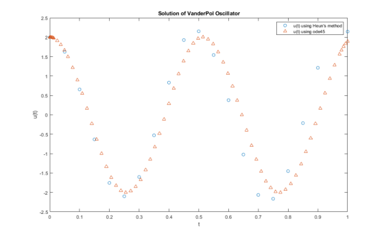
figure, plot(t, u, 'o'), hold on % plotting for part (e)

% Part (d)
[t,y] = ode45(@vdp, [0 1], [u(1); v(1)]);
plot(t, y(:,1), '^'), xlabel('t'), ylabel('u(t)')
title('Solution of VanderPol Oscillator')
legend('u(t) using Heun''s method', 'u(t) using ode45')

function f = func_u(~,~,v) % u'
f = v;
end

function f = func_v(~,u,v) % v'
a = 150; gamma = 1.0;
f = gamma*(1 - u^2)*v - a*u;
end

function dydt = vdp(~,y)
a = 150; gamma = 1.0;
dydt = [y(2);
gamma*(1 - y(1)^2)*y(2) - a*y(1)];
end

Plot:

Solution of VanderPol Oscillator O u(t) using Heun's method A u(t) using ode45 2 1.5 0.5 -0.5 2.5 0.1 0.2 0.3 0.4 0.5 0.6 0.7 0.8 0.9