Homework Answers
clear
clc
close all
s = tf('s');
%definig each block's TF
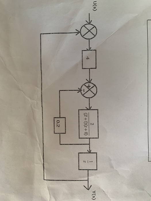
G1 = 4*(1+0*s); %approximating 4
G2 = 2/((s+1)*(s+8));
G3 = 1/s;
G4 = 0.2*(1+0*s); %approximating 0.2
%definig inputs and outputs for each block
G1.InputName = 'r'; G1.OutputName = 'eg1';
G2.InputName = 'e'; G2.OutputName = 'ym';
G3.InputName = 'ym';G3.OutputName = 'y';
G4.InputName = 'ym';G4.OutputName = 'eg4';
%summing points
sum1 = sumblk('r','u','y'); % r = u + y
sum2 = sumblk('e','eg1','eg4','+-'); % e = eg1 - eg4
%connecting the blocks to relate input u with output y
closedLoopTF = connect(G1,G2,G4,G3,sum1,sum2,'u','y');
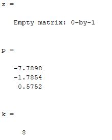
%obtaining zeros z, poles p and gain k
[z,p,k] = zpkdata(closedLoopTF,'v')
COMMENT DOWN FOR ANY QUERY RELATED TO THIS ANSWER,
IF YOU'RE SATISFIED, GIVE A THUMBS UP
~yc~
Add Answer to:
solve it simply by using Matlab first find cloosed loop transfer function second find zeros, poles and gain Y(s) 0 U(s) 2 4 0.2 Y(s) 0 U(s) 2 4 0.2
1) Write a Matlab program for the following block diagram: a) to derive its closed-loop transfer function. b) to find and plot the poles-zeros of closed-loop transfer function. s+2s+3 R(s) → Y(s)...
 1) Write a Matlab program for the following block diagram: a) to derive its closed-loop transfer function. b) to find and plot the poles-zeros of closed-loop transfer function. s+2s+3 R(s) → Y(s) 2s+3 2 +2s +5 15 Automatic Control Systen
1) Write a Matlab program for the following block diagram: a) to derive its closed-loop transfer function. b) to find and plot the poles-zeros of closed-loop transfer function. s+2s+3 R(s) → Y(s) 2s+3 2 +2s +5 15 Automatic Control Systen
1) Write a Matlab program for the following block diagram: a) to derive its closed-loop transfer function. b) to find and plot the poles-zeros of closed-loop transfer function. s+2s+3 R(s) → Y(s) 2s+3 2 +2s +5 15 Automatic Control Systen
For the following systems, find the transfer function using MATLAB. Also, determine the poles and zeros...
 For the following systems, find the transfer function using MATLAB. Also, determine the poles and zeros of each transfer. You should be able to use some combination of the following MATLAB functions: 'ss2tf( )', 'ss( )', 'tf( )', 'pole( )', "zero( )', and 'roots() 100 ).y) = [0_1)|) 2 a. |x2(t)] -10 [x1 (t lx20 21 b. + 01 x1 (t) 0 x2(t) 1 u(t), y(t): ol]x3(t)] [(t)] x2(t) 3(t) [x1 (t)] [o 0 1x2(t) [x3(t)] -4 -2 0 2...
Solve the following using MATLAB: 3. Consider the transfer function: H S ) = 6 2s2...
 Solve the following using MATLAB:
3. Consider the transfer function: H S ) = 6 2s2 + 6s 2s4 + 8 s +3 .4 L + 3 a) Write lines of code to find the zeros and poles of the above transfer function. b) Write lines of code to find a partial fraction expansion of the above transfer function.
Solve the following using MATLAB:
3. Consider the transfer function: H S ) = 6 2s2 + 6s 2s4 + 8 s +3 .4 L + 3 a) Write lines of code to find the zeros and poles of the above transfer function. b) Write lines of code to find a partial fraction expansion of the above transfer function.
a.)Determine the values of the poles and zeros of the closed loop system shown when the controller gain kc = 0. answer should be no zeros poles at s = 2.0 and -0.5 ± j b.) Compare these with the open...
 a.)Determine the values of the
poles and zeros of the closed loop system shown when the controller
gain kc = 0.
answer should be
no zeros
poles at s = 2.0 and -0.5 ± j
b.) Compare these with the open loop poles and zeros.
c.) Now determine the values of the poles and zeros at some very
high gain, say kc = 105 .
Determine the values of the poles and zeros of the closed loop system shown when...
a.)Determine the values of the
poles and zeros of the closed loop system shown when the controller
gain kc = 0.
answer should be
no zeros
poles at s = 2.0 and -0.5 ± j
b.) Compare these with the open loop poles and zeros.
c.) Now determine the values of the poles and zeros at some very
high gain, say kc = 105 .
Determine the values of the poles and zeros of the closed loop system shown when...
Theroot-locus design method (d) Gos)H(s)2) 5.5 Complex poles and zeros. For the systems with an open-loop transfer function given below, sketch the root locus plot. Find the asymptotes and their angle...
 Theroot-locus design method
(d) Gos)H(s)2) 5.5 Complex poles and zeros. For the systems with an open-loop transfer function given below, sketch the root locus plot. Find the asymptotes and their angles. the break-away or break-in points, the angle of arrival or departure for the complex poles and zeros, respectively, and the range of k for closed-loop stability 5 10ん k(s+21
(d) Gos)H(s)2) 5.5 Complex poles and zeros. For the systems with an open-loop transfer function given below, sketch the root...
Theroot-locus design method
(d) Gos)H(s)2) 5.5 Complex poles and zeros. For the systems with an open-loop transfer function given below, sketch the root locus plot. Find the asymptotes and their angles. the break-away or break-in points, the angle of arrival or departure for the complex poles and zeros, respectively, and the range of k for closed-loop stability 5 10ん k(s+21
(d) Gos)H(s)2) 5.5 Complex poles and zeros. For the systems with an open-loop transfer function given below, sketch the root...
alpha = 5.0 beta = 7.1 zeta = 6.9 PROBLEM 1 (20 points). Given the filter with transfer function +28-1+-2 11(2) = 1-(α/10)2-4 (a2/100):-2 Use MATLAB to Find the zeros and poles of H() Plot the pole...
 alpha = 5.0
beta = 7.1
zeta = 6.9
PROBLEM 1 (20 points). Given the filter with transfer function +28-1+-2 11(2) = 1-(α/10)2-4 (a2/100):-2 Use MATLAB to Find the zeros and poles of H() Plot the poles and zeros on the -plane. The pot should include the uit circle. Plot the magnitude response (in dB) Plot the phase response. Deliverables: Your MATLAB code used to solve Problem 1 and all the generated plots.
PROBLEM 1 (20 points). Given the filter...
alpha = 5.0
beta = 7.1
zeta = 6.9
PROBLEM 1 (20 points). Given the filter with transfer function +28-1+-2 11(2) = 1-(α/10)2-4 (a2/100):-2 Use MATLAB to Find the zeros and poles of H() Plot the poles and zeros on the -plane. The pot should include the uit circle. Plot the magnitude response (in dB) Plot the phase response. Deliverables: Your MATLAB code used to solve Problem 1 and all the generated plots.
PROBLEM 1 (20 points). Given the filter...
4. Determine the transfer function, poles and zeros, and stability of the system represented by the...
4. Determine the transfer function, poles and zeros, and stability of the system represented by the following difference equation: y[n] = -1.5y[n-1] + y[n-2] + x[n] Answers:H[z]= 1/(1+(1.5z^-1) - (z^-2)); poles at z = -2, 0, 5; zeros at z=0; unstable
105- Problem #4 - Given the transfer function T(s)- ***(1+%o1+%0011+%00) A) Find the Poles and Zeros....
 105- Problem #4 - Given the transfer function T(s)- ***(1+%o1+%0011+%00) A) Find the Poles and Zeros. B) Sketch the Bode plots for the magnitude and phase of the function. C) From the plot estimate the gain and phase at 1000 rad/s and compare to actual calculated values.
1. (20 points). A transfer function has the following zeros and poles: zero at s=-105 and s= poles at s-100 and s--1000. The magnitude of the transfer function at ω= 105 rad/s is equal 100. Find the...
 1. (20 points). A transfer function has the following zeros and poles: zero at s=-105 and s= poles at s-100 and s--1000. The magnitude of the transfer function at ω= 105 rad/s is equal 100. Find the transfer function T(s) and sketch Bode plots for the magnitude and phase, ˇ
1. (20 points). A transfer function has the following zeros and poles: zero at s=-105 and s= poles at s-100 and s--1000. The magnitude of the transfer function at ω=...
1. (20 points). A transfer function has the following zeros and poles: zero at s=-105 and s= poles at s-100 and s--1000. The magnitude of the transfer function at ω= 105 rad/s is equal 100. Find the transfer function T(s) and sketch Bode plots for the magnitude and phase, ˇ
1. (20 points). A transfer function has the following zeros and poles: zero at s=-105 and s= poles at s-100 and s--1000. The magnitude of the transfer function at ω=...
Given ℎ(t) = (e-t + e-2t) u(t) find: a) H(s) transfer function b) Poles and Zeros...
Given ℎ(t) = (e-t + e-2t) u(t) find: a) H(s) transfer function b) Poles and Zeros location c) System stable or unstable? d) Differential Equation associated with the system
 1) Write a Matlab program for the following block diagram: a) to derive its closed-loop transfer function. b) to find and plot the poles-zeros of closed-loop transfer function. s+2s+3 R(s) → Y(s) 2s+3 2 +2s +5 15 Automatic Control Systen
1) Write a Matlab program for the following block diagram: a) to derive its closed-loop transfer function. b) to find and plot the poles-zeros of closed-loop transfer function. s+2s+3 R(s) → Y(s) 2s+3 2 +2s +5 15 Automatic Control Systen
1) Write a Matlab program for the following block diagram: a) to derive its closed-loop transfer function. b) to find and plot the poles-zeros of closed-loop transfer function. s+2s+3 R(s) → Y(s) 2s+3 2 +2s +5 15 Automatic Control Systen
 For the following systems, find the transfer function using MATLAB. Also, determine the poles and zeros of each transfer. You should be able to use some combination of the following MATLAB functions: 'ss2tf( )', 'ss( )', 'tf( )', 'pole( )', "zero( )', and 'roots() 100 ).y) = [0_1)|) 2 a. |x2(t)] -10 [x1 (t lx20 21 b. + 01 x1 (t) 0 x2(t) 1 u(t), y(t): ol]x3(t)] [(t)] x2(t) 3(t) [x1 (t)] [o 0 1x2(t) [x3(t)] -4 -2 0 2...
 Solve the following using MATLAB:
3. Consider the transfer function: H S ) = 6 2s2 + 6s 2s4 + 8 s +3 .4 L + 3 a) Write lines of code to find the zeros and poles of the above transfer function. b) Write lines of code to find a partial fraction expansion of the above transfer function.
Solve the following using MATLAB:
3. Consider the transfer function: H S ) = 6 2s2 + 6s 2s4 + 8 s +3 .4 L + 3 a) Write lines of code to find the zeros and poles of the above transfer function. b) Write lines of code to find a partial fraction expansion of the above transfer function.
 a.)Determine the values of the
poles and zeros of the closed loop system shown when the controller
gain kc = 0.
answer should be
no zeros
poles at s = 2.0 and -0.5 ± j
b.) Compare these with the open loop poles and zeros.
c.) Now determine the values of the poles and zeros at some very
high gain, say kc = 105 .
Determine the values of the poles and zeros of the closed loop system shown when...
a.)Determine the values of the
poles and zeros of the closed loop system shown when the controller
gain kc = 0.
answer should be
no zeros
poles at s = 2.0 and -0.5 ± j
b.) Compare these with the open loop poles and zeros.
c.) Now determine the values of the poles and zeros at some very
high gain, say kc = 105 .
Determine the values of the poles and zeros of the closed loop system shown when...
 Theroot-locus design method
(d) Gos)H(s)2) 5.5 Complex poles and zeros. For the systems with an open-loop transfer function given below, sketch the root locus plot. Find the asymptotes and their angles. the break-away or break-in points, the angle of arrival or departure for the complex poles and zeros, respectively, and the range of k for closed-loop stability 5 10ん k(s+21
(d) Gos)H(s)2) 5.5 Complex poles and zeros. For the systems with an open-loop transfer function given below, sketch the root...
Theroot-locus design method
(d) Gos)H(s)2) 5.5 Complex poles and zeros. For the systems with an open-loop transfer function given below, sketch the root locus plot. Find the asymptotes and their angles. the break-away or break-in points, the angle of arrival or departure for the complex poles and zeros, respectively, and the range of k for closed-loop stability 5 10ん k(s+21
(d) Gos)H(s)2) 5.5 Complex poles and zeros. For the systems with an open-loop transfer function given below, sketch the root...
 alpha = 5.0
beta = 7.1
zeta = 6.9
PROBLEM 1 (20 points). Given the filter with transfer function +28-1+-2 11(2) = 1-(α/10)2-4 (a2/100):-2 Use MATLAB to Find the zeros and poles of H() Plot the poles and zeros on the -plane. The pot should include the uit circle. Plot the magnitude response (in dB) Plot the phase response. Deliverables: Your MATLAB code used to solve Problem 1 and all the generated plots.
PROBLEM 1 (20 points). Given the filter...
alpha = 5.0
beta = 7.1
zeta = 6.9
PROBLEM 1 (20 points). Given the filter with transfer function +28-1+-2 11(2) = 1-(α/10)2-4 (a2/100):-2 Use MATLAB to Find the zeros and poles of H() Plot the poles and zeros on the -plane. The pot should include the uit circle. Plot the magnitude response (in dB) Plot the phase response. Deliverables: Your MATLAB code used to solve Problem 1 and all the generated plots.
PROBLEM 1 (20 points). Given the filter...
 105- Problem #4 - Given the transfer function T(s)- ***(1+%o1+%0011+%00) A) Find the Poles and Zeros. B) Sketch the Bode plots for the magnitude and phase of the function. C) From the plot estimate the gain and phase at 1000 rad/s and compare to actual calculated values.
 1. (20 points). A transfer function has the following zeros and poles: zero at s=-105 and s= poles at s-100 and s--1000. The magnitude of the transfer function at ω= 105 rad/s is equal 100. Find the transfer function T(s) and sketch Bode plots for the magnitude and phase, ˇ
1. (20 points). A transfer function has the following zeros and poles: zero at s=-105 and s= poles at s-100 and s--1000. The magnitude of the transfer function at ω=...
1. (20 points). A transfer function has the following zeros and poles: zero at s=-105 and s= poles at s-100 and s--1000. The magnitude of the transfer function at ω= 105 rad/s is equal 100. Find the transfer function T(s) and sketch Bode plots for the magnitude and phase, ˇ
1. (20 points). A transfer function has the following zeros and poles: zero at s=-105 and s= poles at s-100 and s--1000. The magnitude of the transfer function at ω=...
Most questions answered within 3 hours.
-
Where is the error in this code sequence?
String s1 = "Hello";
String s2 = "ello";...
asked 11 months ago -
Financial data for Joel de Paris, Inc., for last year
follow:
Joel de Paris, Inc.
Balance...
asked 11 months ago -
Consider this reaction:
Al2(SO4)3 (aq)+ BaCl3
(aq) Al2Cl6 (aq)- +
3BaSO4(s) . What is the...
asked 11 months ago -
Suppose that Savneet is considering increasing her
recent random sample from 20 car rentals to 40...
asked 11 months ago -
Trucks arrive at an unloading terminal at an average rate of 120
per hour.
Trucks arrive...
asked 11 months ago -
Why are methanol and ethanol completely soluble in water while
octanol is not very little soluble....
asked 11 months ago -
A facilities manager at a university reads in a research report
that the mean amount of...
asked 11 months ago -
When the CuSO4 is rehydrated by adding water to the anhydrous
compound, is this an endothermic...
asked 11 months ago -
A ray of sunlight is passing from diamond into crown glass; the
angle of incidence is...
asked 11 months ago -
A block of mass 0.249 kg is placed on top of a light, vertical
spring of...
asked 11 months ago -
how do the kidneys compensate in the presences of acidosis
a) trigger hyperventilate
b) reserve acid...
asked 11 months ago -
Question 501 pts
The rental rate of capital to the firm increases. Which of the
following...
asked 11 months ago