Question

4. Let x- be a two dimensional feature vector (a) Suppose that we collect the following four measurements for an input belonging to class a x1 -6 -10 10 -6 Assuming that the class conditional density is Gaussian, find the maximum likelihood estimates of the mean vector and covariance matrix for class ω (b) Suppose that data come from two classes, a, and co,. Assume that . The a priori class probabilities are equal . The class conditional densities are Gaussian The mean vector and covariance matrix of class are the same as computed in (a) The covariance matrix ofclass a), is the same as that of class a, but the mean vector is given . the classes are equally likely. Find the formula for the decision boundary separating the two classes if you use a Bayes classifier. Plot the decision boundary in the (x, ) plane. (c) Find the formula for and plot the decision boundary if the a priori class probabilities change so that P(a) 0.3

Answer 1

(a) The data vector is

T1 2

Given that the class conditional density is Gaussian.

The maximum likelihood estimate for mean vector is expressed as

3 7721 106 10 6 に!

8 2 3

The maximum likelihood estimate for co-variance matrix is expressed as

k=1

4 2 2 4 2 2

4 0 0 1 40

=================================================================

(b) The first point states that
lun
because $p(\omega_1) + p(\omega_2) =1$

The second and the third point states that

m1-
and
4 0

The fourth point states that

$m_2 = \begin{bmatrix} 1\\1 \end{bmatrix}$ and $\Sigma_2 = \begin{bmatrix} 1 & 0\\ 0 & 4 \end{bmatrix}$

Applying Bayes classifier for two classes, the decision boundary $p(\omega_1|x) >= p(\omega_2|x)$

The linear discriminant function is simplified as

$g_1(x) = \log p(x|\omega_1) + \log p(\omega_1)$ and

92()logp(rw)+log p(2)

Using Gaussian density, the linear discriminant function reduces to form of

$g_1(x) = \omega_1^{T}x + \omega_{10}$

where

$\omega_1 = \Sigma_1^{-1}m_1$

and $\omega_{10} = -\frac{1}{2}m_1 \Sigma_1^{-1}m_1 + \log p(\omega_1)$

$g_2(x) = \omega_2^{T}x + \omega_{20}$

where

$\omega_2 = \Sigma_2^{-1}m_2$

and $\omega_{20} = -\frac{1}{2}m_2 \Sigma_2^{-1}m_2 + \log p(\omega_2)$

The decision boundary is expressed as

which simplifies to $\omega^{T}(x-x_0) = 0$

where,

$\omega = \Sigma^{-1}(m_1 - m_2)$

and

$x_0 = \frac{1}{2} (m_1 + m_2) - \frac{\log [p(\omega_1)/p(\omega_2)]}{(m_1-m_2)^{T}\Sigma^{-1}(m_1 - m_2)}(m_1-m_2)$

The second term in the above expression is zero because

lun

Therefore, $x_0 = \frac{1}{2} (m_1 + m_2) = \frac{1}{2}\left ( \begin{bmatrix} 2\\ -8 \end{bmatrix} + \begin{bmatrix} 1\\ 1 \end{bmatrix} \right ) = \frac{1}{2}\left ( \begin{bmatrix} 3\\ -7 \end{bmatrix} \right ) = \begin{bmatrix} 1.5\\ -3.5 \end{bmatrix}$

$\omega = \Sigma^{-1}(m_1 - m_2) = \begin{bmatrix} 1 &0 \\ 0 & 0.25 \end{bmatrix} \begin{bmatrix} 1\\ -9 \end{bmatrix} = \begin{bmatrix} 1\\ -2.25 \end{bmatrix}$

Substituting $\omega$ and $x_0$ in the equation $\omega^{T}(x-x_0) = 0$ , we get

](12.11-11.5 T2-3.5 1 -2.25

The above expression is the required decision boundary

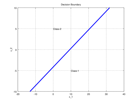
Let us calculate different values for $x_1$ in terms of $x_2$ using the above equation as

Taking different values for $x_2$ from -10 to 10 in steps of 1. We get a plot as shown below,

Decision Boundary 10 Class-2 Class-t -5 -10 -20 10 20 40 30 -10

=================================================================

(c) The prior class probability changes with $p(\omega_1) = 0.3$ and thus, $p(\omega_2) = 0.7$

$\omega = \Sigma^{-1}(m_1 - m_2)$

and

$x_0 = \frac{1}{2} (m_1 + m_2) - \frac{\log [p(\omega_1)/p(\omega_2)]}{(m_1-m_2)^{T}\Sigma^{-1}(m_1 - m_2)}(m_1-m_2)$

In the above equations, $\omega$ remains same, but $x_0$ changes due in $p(\omega_1)$ and $p(\omega_2)$.

Calculating $x_0$ again,

1.5 | log|0.3/0.7] TO-3.52 1.5399 3.5 +0.039873 21.250 -9 9-3.8589

Substituting $\omega$ and $x_0$ in the equation $\omega^{T}(x-x_0) = 0$ , we get

$\begin{bmatrix} 1 & -2.25 \end{bmatrix}\left ( \begin{bmatrix} x_1\\ x_2 \end{bmatrix} - \begin{bmatrix} 1.5399\\-3.8589 \end{bmatrix}\right ) = 0$

The above expression is the required decision boundary

Let us calculate different values for $x_1$ in terms of $x_2$ using the above equation as

Taking different values for $x_2$ from -10 to 10 in steps of 1. We get a plot as shown below,

================================================================

Decision Boundary 10 Class-2 Class-t -5 -10 -20 10 20 40 30 -10

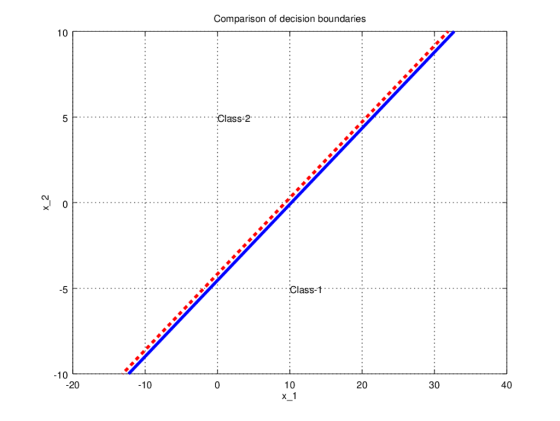
Note: We need to compare the decision boundaries between the two problems for change in prior class probabilities. The combined plot is shown below, the red dash line shows the earlier decision boundary and the blue line shows the new decision boundary. It can be thought as the red line is shifted down wards to the blue line due to reduction the prior class probability for Class-1.

Comparison of decision boundaries 10 Class-2 Class-t -5 -10 -20 10 20 40 30 -10