Question

2. (37 points) The manager of a travel agency wants to use seasonally adjusted forecast to predict demand for packaged tours. The demand for the last 14 weeks are given below: Week 1 2 3 4 5 6 7 89 10 1112 13 14 Demand 80 95 141 132 104 114 168 152 122 143 198 185 141 158 (10 points) Estimate weekly relatives for the demand using the centered moving average method. (10 points) Estimate weekly relatives for the demand using the SA method. (5 points) Select your estimates either in (a) or (b). Deseasonalize the data. (5 points) Estimate the trend equation using the deseasonalized data from part (d). (7 points) Forecast demand for weeks 15 and 16. a. b. c. d. e.

Answer 1

In the time series chart, we observe that demand is seasonal and the cycle repeats every 4 weeks.

EXCEL FORMULAS:

Seasonal Dt/Ct Line Trend FORECAST(B3,SH$3 SH$ 4-period MA Deseasonalized Period Week Demand (Dt) Simple Centered (Ct) St Forecast St VLOOKUP A3,SD$21 $F$25,3,0)C3/G3 VLOOKUP A4,SD$21:SF$25,3,0 VLOOKUPIAS SD$21:SF$25,3,0) VLOOKUP A5,SD$21 $F$25,3,0C6/G6 VLOOKUPIA7,SD$21:SF$25,3,0) 80 -C4 FORECAST(84,S S S -c5/ES -C6/E6 141 -FORECAST BS,SHS3:SHS -FORECAST(B6,SH$3 SHS AVERAGEC4:C7) AVE AVERAGEC6:09 AVERAGE C7:C10) AVERAGE D6:07 AVERAGE D7:D8 AVERAGE D8:D9 AVERAGE D9:010) 104 CS:C8 -FORECAST B7,SHS3:SH C8/E8 C9 тва,SHS3 SH$3 152 122 143 198 185 141 158 VLOOKUP A9,SD$21 $F$25,3,0) VLOOKUPIA10,SDS21:SFS25,3,0 VLOOKUPIA11,SDS21:SFS25,3,0)C11/G11 VLOOKUP A12.$D$21 $F$25,3,0)C12/G12 VLOOKUPIA13,SDS21 $F$25,3,0) C13/G13 VLOOKUP A14SDS21 $FS25,3,0)C14/G14 VLOOKUP A15 VLOOKUPIA16,SDS21:SFS25,3,0) C16/G16 VLOOKUP(A17,ŞD$21:$F$25,3,0) VLOOKUP(A18,SD$21:SF$25,3,0) FORECAST B9,$ $ $ =FORECAST( B10,SHS -FORECAST(B11,SHS3:$H FORECAST B12,5H$3 $H FORECAST(B13,SH$3:$H -FORECAST (B14.SHS3 $H -FORECAST B15,SH$3 -FORECAST(B16,SHS3:SH -FORECAST(B17,$H$3:$ FORECASTB18,SHS3:S 10 4 AVERAGEIC8C11)AVERAGE D10:011) AVERAGEC9:C12 AVERAGE(D11:D12) AVERAGE C10 C13) AVERAGE D12:D13) AVERAGE(C11:C14) FAVERAGE D13:D14) AVERAGE(C12:C15) |-AVERAGE(D14:D15) AVERAGEC13:C16) -C10/G10 -C11/E11 C12/E12 C13/E13 C14/E14 12 2 16 2 20 Period Unadjusted Seasonal relative Adjusted Seasonal relative AVERAGEIFISA$3:$A$16,D22,SF$3:$F$16)FE22/SE$26 COUNTISE$22 SE$25) AVERAGEIFISAS3:ŞAS16,D23,SF$3 SFS16) E23/SEŞ26 COUNTISEŞ22:SEŞ25) AVERAGEIFISAS3 $A$16,D24,SF$3 $F$16)E24/SE$26 COUNTISES22 SE$25) AVERAGEIFISA$3:$A$16,D25,SF$3 ŞF$16 E25/SE$26 COUNTISE$22 SE$25) -SUM(E22:E25 26 Total SUM (F22:F25

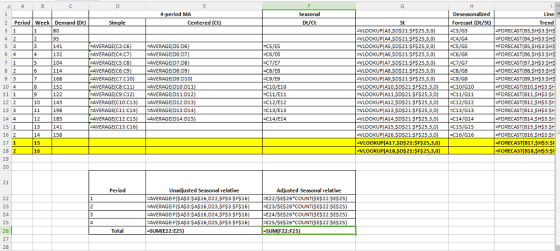
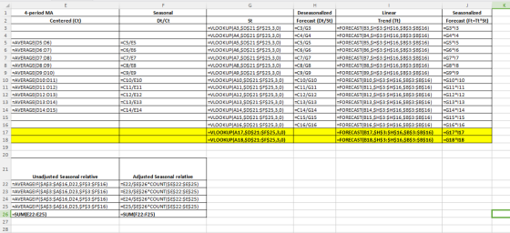
a) Weekly relatives are:

Period	Adjusted Seasonal relative
1	0.8169
2	0.8825
3	1.2167
4	1.0838

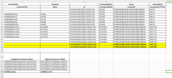
b) Weekly relatives are determined using SA (simple average) method as below

c) Deseasonalized forecast is shown in column H

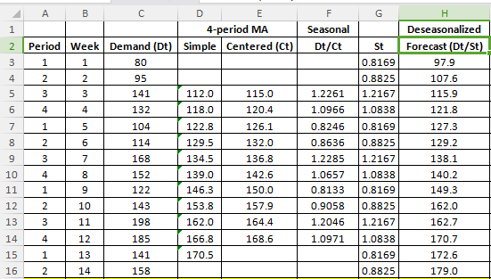
d) Trend equation for deseasonalized data can be determined by formulas:

Slope =SLOPE(H3:H16,B3:B16) = 6.1208

Intercept =INTERCEPT(H3:H16,B3:B16) = 95.1276

Trend equation is:

y = 95.1276 + 6.1208*x , where x is trend forecast and x is week iindex

e)

Forecase demand for week 15 and 16 is calculated in column J

Forecast for week 15 = 153

Forecas for week 16 = 170

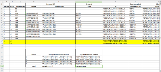
FORMULA VIEW: