Question

can i get some help on this question please, thanks!

The values below shows the number of new stores in a coffee shop chain that opened during the years 1986 through 1994. 1986, 14 1987, 27 1988, 48 1989, 80 1990, 110 1991, 153 1992, 261 1993, 403 1994, 681 Use your TI to create two lists L1 for year, L2 for number of new stores. Then create a third list L3 which takes Ln(L2) -- the natural log of L2 Run two LinRegTTest and a) Compute the linear correlation between lists L1 and L2, and the p-value with conclusion, what is the linear regression line. How many new stores do you anticipate in 1995 using this model? b) Compute the exponential correlation between lists L1 and L3 and the p-value with conclusion, what is the exponential regression function. How many new stores do you anticipate in 1995 using this model? c) which model is the better fit?

Answer 1

First we need to create two lists L1 and L2 in TI 84-Plus calculator

Command: Click on STAT >>> 1: Edit

Select L1 and then click on CLEAR

Then enter the given values of first column one by one.

Then select L2 using arrow button

Then enter the given values of second column one by one.

Then select L3

and click on LN >>> 2ND >>> 2 >>> ENTER

So we get the values of L3

Now, we need to run Linear regression test:

Command:

STAT >>> TESTS >>> F : LinRegTTest...ENTER

Look the following image:

Wabbitemu X File View Calculator Debug Help TI-84 Plus Silver Edition TEXAS INSTRUMENTS LinRe3TTest Xlist:L1 Y1ist:Lz Freq: 1 B & PE<G 0 RegEQ: Calculate STAT PLOT F1 TBLSET F2 FORMAT F3 TABLE F CALC F4 GRAPH WINDOW TRACE ZOOM QUIT 2ND MODE DEL ALOCK LINH ALPHA ΧΤ,θη STAT TEST ANGLE B DRAW C MATH CLEAR VARS APPS PRGM COS 1 F TAN-1 G x- SIN TAN cos EE I LOG 7 8 L4 T LS U L6 V LN 4 6 5 STO 12 Z TRY SOLVE 1 3 2 ENTER ON CATALOG ANS (-) OD

Select the input like above image and click on ENTER

So we get the following output

TI-84 Plus Silver Edition TEXAS INSTRUMENTS LinR3TTst yHa+bx B 0 and Pr0 t=5.150781326 R=.0013228647 df 7 a=-142253.3889 STAT PLOT F1 TBLSET F2 FORMAT F3 YoWINDOW TABLE FS CALC F4 TRACE GRAPH ZOOM

Then using down arrow button we get the remaining output as follows:

S TI-84 Plus Silver Edition TEXAS INSTRUMENTS LinR 3TTst yIa+bx B+Oand P tb-71.58333333 s=107.6500982 r.7912351464 r=.8895139945 STAT PLOT F1 TBLSET F2 FORMAT F3 ZOOM CALC F4 TABLE F Y WINDOW GRAPH TRACE

From the above output the linear correlation coefficients ( r ) of L1 and L2 is as follows:

r = 0.8895

and p-value = 0.0013

Decision rule:

1) If p-value < level of significance (alpha) then we reject null hypothesis

2) If p-value > level of significance (alpha) then we fail to reject null hypothesis.

Here p value = 0.0013 < 0.05 so we used first rule.

That is we reject null hypothesis

Conclusion: At 5% level of significance there are not sufficient evidence to conclude that the correlation between L1 and L2 is linear.

The linear regression line of L2 on L1 is as follows:

y = a + bx

y = -142253.3889 + 71.5833 x

Let's plug x = 1995 in the above model, we get:

y =-142253.3889+(71.5833* 1995 ) = 555.29 which is approximately equal to 555.

b) Similarly do the regression between L1 and L3

so we get the following result:

Wabbitemu File View Calculator Debug Help TI-84 Plus Silver Edition TEXAS INSTRUMENTS LinRe3TTest yHa+bx B#0 and Pt t-30.69628279 P 1.0050173E-8 df=7 a-913.4645677 STAT PLOT F1 TB LSET F2 FORMAT F3 CALC F4 TABLE FS ZOOM Y WINDOW TRACE GRAPH X

Wabbitemu File View Calculator Debug Help TI-84 Plus Silver Edition TEXAS INSTRUMENTS LinReSTTest ya+bx B 0 and P+0 tb=.4613728179 s.1164238193 r.9926258487 r-.9963061019 STAT PLOT F1 TB LSET F2 FORMAT F3 CALC F4 TABLE FS Y WINDOW Z0OM GRAPH TRACE X

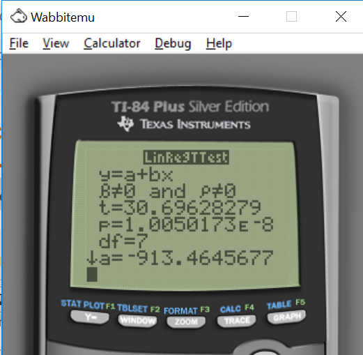
From the above output the linear correlation coefficients ( r ) of L1 and L3 is as follows:

r = 0.9963

and p-value = 0.00

Decision rule:

1) If p-value < level of significance (alpha) then we reject null hypothesis

2) If p-value > level of significance (alpha) then we fail to reject null hypothesis.

Here p value = 0.0 < 0.05 so we used first rule.

That is we reject null hypothesis

Conclusion: At 5% level of significance there are not sufficient evidence to conclude that the correlation between L1 and L3 is linear.

The linear regression line of L3 on L1 is as follows:

y = a + bx

y = -913.46 + 0.4614 x

Let's plug x = 1995 in the above model, we get:

y = -913.46 + (0.4614*1995) = 7.033

y = 7.033

Taking exponential of 7.033, we get

y = 1133.43 = 1133

The model in part b ) is better because the value of r in part b) is large than the value of r in part a).