

Homework Answers

Add Answer to:
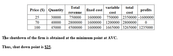
5. Profit maximization and shutting down in the short run Suppose that the market for blenders...
5. Profit maximization and shutting down in the short run Suppose that the market for black...
 5. Profit maximization and shutting down in the short run Suppose that the market for black leather purses is a competitive market. The following graph shows the daily cost curves of a firm operating in this market. PRICE (Dollars per purse) + MC AVC 0 10 90 100 20 30 40 50 60 70 80 QUANTITY (Thousands of purses) For each price in the following table, calculate the firm's optimal quantity of units to produce, and determine the profit or...
4. Short-run profit maximization or loss minimization for a perfectly competitive firm Suppose that the market...
 4. Short-run profit maximization or loss minimization for a perfectly competitive firm Suppose that the market for cashmere sweaters is a perfectly competitive market. The following graph shows the daily cost curves of a firm operating in this market. Profit or Loss PRICE AND COST (Dollars per sweater) 0 10 90 100 20 30 40 50 60 70 80 QUANTITY OF OUTPUT (Sweaters) In the short run, at a market price of $80 per sweater, this firm will choose to...
6. Deriving the short-run supply curve Consider the competitive market for halogen lamps. The following graph...
 6. Deriving the short-run supply curve Consider the competitive market for halogen lamps. The following graph shows the marginal cost (MC), average total cost (ATC), and average variable cost (AVC) curves for a typical firm in the industry. 90 80 6 2 50 3 40 30 AVC 10 20 30 40 50 70 100 QUANTITY Thousands of lamps)
6. Deriving the short-run supply curve Consider the competitive market for halogen lamps. The following graph...
 6. Deriving the short-run supply curve Consider the competitive market for halogen lamps. The following graph shows the marginal cost (MC), average total cost (ATC), and average variable cost (AVC) curves for a typical firm in the industry. COSTS (Dollars) AVC МСП OHH 0 10 90 100 20 30 40 50 60 70 80 QUANTITY (Thousands of lamps) On the following graph, use the orange points (square symbol) to plot points along the portion of the firm's short-run supply curve...
Suppose the competitive market for cat toys is in short-run equilibrium. The following graph on the...
 Suppose the competitive market for cat toys is in short-run equilibrium. The following graph on the left shows the demand and short-run supply for cat toys. Assume every firm in this industry is identical. The graph on the right shows the marginal cost (MC) and average cost (AC) curves for each firm in the long run. Short-Run Market Individual Firm PRICE (Dollars per cat toy) COST (Dollars per cat toy) Supply MC 0 Demand + + + + 0 10...
5. Moving from short-run to long-run equilibrium Suppose the competitive market for cat toys is in...
 5. Moving from short-run to long-run equilibrium Suppose the competitive market for cat toys is in short-run equilibrium. The following graph on the left shows the demand and short-run supply for cat toys. Assume every firm in this industry is identical. The graph on the right shows the marginal cost (MC) and average cost (AC) curves for each firm in the long run. ? ? Short-Run Market Individual Firm 10 10 8 8 AC MC Supply 2 1 1 Demand...
6. Deriving the short-run supply curve Consider the competitive market for halogen lamps. The following graph...
 6. Deriving the short-run supply curve Consider the competitive market for halogen lamps. The following graph shows the marginal cost (MC), average total cost (ATC), and average variable cost (AVC) curves for a typical firm in the industry. COSTS (Dollars) DAVC МСП 0 10 90 100 20 30 40 50 60 70 80 QUANTITY (Thousands of lamps) We were unable to transcribe this imageWe were unable to transcribe this imageWe were unable to transcribe this image
7. Short-run supply and long-run equillbrium Consider the competitive market for steel. Assume that, regardless of...
 7. Short-run supply and long-run equillbrium Consider the competitive market for steel. Assume that, regardless of how many firms are in the industry, every firm in the industry is identical and faces the marginal cost (MC), average total cost (ATC), and average variable cost (AVC) curves shown on the following graph 100 90 27.5, 70 80 70 30 20 AVC 10 0s10 1520 25 30 35 40 45 QUANTITY (Thousands of tons) The following diagram shows the market demand for...
please complete the LR line 3. Moving from short-run to long-run equilibrium Suppose the competitive market...
 please complete the LR line
3. Moving from short-run to long-run equilibrium Suppose the competitive market for cat toys is in short-run equilibrium. The following graph on the left shows the demand and short-run supply for cat toys. Assume every firm in this industry is identical. The graph on the right shows the marginal cost (MC) and average cost (AC) curves for each firm in the long run. Short-Run Market Individual Firm Supply PRICE (Dollars per cat toy) AAAAAAAA+ COST...
please complete the LR line
3. Moving from short-run to long-run equilibrium Suppose the competitive market for cat toys is in short-run equilibrium. The following graph on the left shows the demand and short-run supply for cat toys. Assume every firm in this industry is identical. The graph on the right shows the marginal cost (MC) and average cost (AC) curves for each firm in the long run. Short-Run Market Individual Firm Supply PRICE (Dollars per cat toy) AAAAAAAA+ COST...
6. Short-run perfectly competitive equilibrium Consider a perfectly competitive market for wheat in Philadelphia. There...
 6. Short-run perfectly competitive equilibrium Consider a perfectly competitive market for wheat in Philadelphia. There are 80 firms in the industry, each of which has the cost curves shown on the following graph: MC ATC COST (Cents per bushel) AVC 0 5 10 15 20 25 30 35 40 45 50 Demand Supply Curve Equilibrium PRICE (Cents per bushel) 0 400 800 1200 1600 2000 2400 2800 3200 3600 4000 QUANTITY OF OUTPUT (Thousands of bushels) in the short run....
 5. Profit maximization and shutting down in the short run Suppose that the market for black leather purses is a competitive market. The following graph shows the daily cost curves of a firm operating in this market. PRICE (Dollars per purse) + MC AVC 0 10 90 100 20 30 40 50 60 70 80 QUANTITY (Thousands of purses) For each price in the following table, calculate the firm's optimal quantity of units to produce, and determine the profit or...
 4. Short-run profit maximization or loss minimization for a perfectly competitive firm Suppose that the market for cashmere sweaters is a perfectly competitive market. The following graph shows the daily cost curves of a firm operating in this market. Profit or Loss PRICE AND COST (Dollars per sweater) 0 10 90 100 20 30 40 50 60 70 80 QUANTITY OF OUTPUT (Sweaters) In the short run, at a market price of $80 per sweater, this firm will choose to...
 6. Deriving the short-run supply curve Consider the competitive market for halogen lamps. The following graph shows the marginal cost (MC), average total cost (ATC), and average variable cost (AVC) curves for a typical firm in the industry. 90 80 6 2 50 3 40 30 AVC 10 20 30 40 50 70 100 QUANTITY Thousands of lamps)
 6. Deriving the short-run supply curve Consider the competitive market for halogen lamps. The following graph shows the marginal cost (MC), average total cost (ATC), and average variable cost (AVC) curves for a typical firm in the industry. COSTS (Dollars) AVC МСП OHH 0 10 90 100 20 30 40 50 60 70 80 QUANTITY (Thousands of lamps) On the following graph, use the orange points (square symbol) to plot points along the portion of the firm's short-run supply curve...
 Suppose the competitive market for cat toys is in short-run equilibrium. The following graph on the left shows the demand and short-run supply for cat toys. Assume every firm in this industry is identical. The graph on the right shows the marginal cost (MC) and average cost (AC) curves for each firm in the long run. Short-Run Market Individual Firm PRICE (Dollars per cat toy) COST (Dollars per cat toy) Supply MC 0 Demand + + + + 0 10...
 5. Moving from short-run to long-run equilibrium Suppose the competitive market for cat toys is in short-run equilibrium. The following graph on the left shows the demand and short-run supply for cat toys. Assume every firm in this industry is identical. The graph on the right shows the marginal cost (MC) and average cost (AC) curves for each firm in the long run. ? ? Short-Run Market Individual Firm 10 10 8 8 AC MC Supply 2 1 1 Demand...
 6. Deriving the short-run supply curve Consider the competitive market for halogen lamps. The following graph shows the marginal cost (MC), average total cost (ATC), and average variable cost (AVC) curves for a typical firm in the industry. COSTS (Dollars) DAVC МСП 0 10 90 100 20 30 40 50 60 70 80 QUANTITY (Thousands of lamps) We were unable to transcribe this imageWe were unable to transcribe this imageWe were unable to transcribe this image
 7. Short-run supply and long-run equillbrium Consider the competitive market for steel. Assume that, regardless of how many firms are in the industry, every firm in the industry is identical and faces the marginal cost (MC), average total cost (ATC), and average variable cost (AVC) curves shown on the following graph 100 90 27.5, 70 80 70 30 20 AVC 10 0s10 1520 25 30 35 40 45 QUANTITY (Thousands of tons) The following diagram shows the market demand for...
 please complete the LR line
3. Moving from short-run to long-run equilibrium Suppose the competitive market for cat toys is in short-run equilibrium. The following graph on the left shows the demand and short-run supply for cat toys. Assume every firm in this industry is identical. The graph on the right shows the marginal cost (MC) and average cost (AC) curves for each firm in the long run. Short-Run Market Individual Firm Supply PRICE (Dollars per cat toy) AAAAAAAA+ COST...
please complete the LR line
3. Moving from short-run to long-run equilibrium Suppose the competitive market for cat toys is in short-run equilibrium. The following graph on the left shows the demand and short-run supply for cat toys. Assume every firm in this industry is identical. The graph on the right shows the marginal cost (MC) and average cost (AC) curves for each firm in the long run. Short-Run Market Individual Firm Supply PRICE (Dollars per cat toy) AAAAAAAA+ COST...
 6. Short-run perfectly competitive equilibrium Consider a perfectly competitive market for wheat in Philadelphia. There are 80 firms in the industry, each of which has the cost curves shown on the following graph: MC ATC COST (Cents per bushel) AVC 0 5 10 15 20 25 30 35 40 45 50 Demand Supply Curve Equilibrium PRICE (Cents per bushel) 0 400 800 1200 1600 2000 2400 2800 3200 3600 4000 QUANTITY OF OUTPUT (Thousands of bushels) in the short run....
Most questions answered within 3 hours.
-
Where is the error in this code sequence?
String s1 = "Hello";
String s2 = "ello";...
asked 10 months ago -
Financial data for Joel de Paris, Inc., for last year
follow:
Joel de Paris, Inc.
Balance...
asked 10 months ago -
Consider this reaction:
Al2(SO4)3 (aq)+ BaCl3
(aq) Al2Cl6 (aq)- +
3BaSO4(s) . What is the...
asked 10 months ago -
Suppose that Savneet is considering increasing her
recent random sample from 20 car rentals to 40...
asked 10 months ago -
Trucks arrive at an unloading terminal at an average rate of 120
per hour.
Trucks arrive...
asked 10 months ago -
Why are methanol and ethanol completely soluble in water while
octanol is not very little soluble....
asked 10 months ago -
A facilities manager at a university reads in a research report
that the mean amount of...
asked 10 months ago -
When the CuSO4 is rehydrated by adding water to the anhydrous
compound, is this an endothermic...
asked 10 months ago -
A ray of sunlight is passing from diamond into crown glass; the
angle of incidence is...
asked 10 months ago -
A block of mass 0.249 kg is placed on top of a light, vertical
spring of...
asked 10 months ago -
how do the kidneys compensate in the presences of acidosis
a) trigger hyperventilate
b) reserve acid...
asked 10 months ago -
Question 501 pts
The rental rate of capital to the firm increases. Which of the
following...
asked 10 months ago