
Homework Answers

Add Answer to:
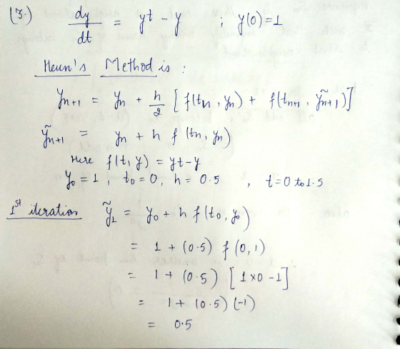
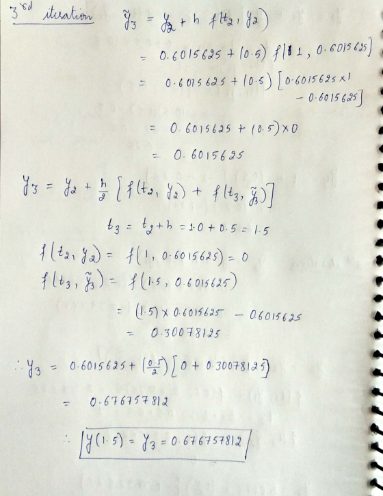
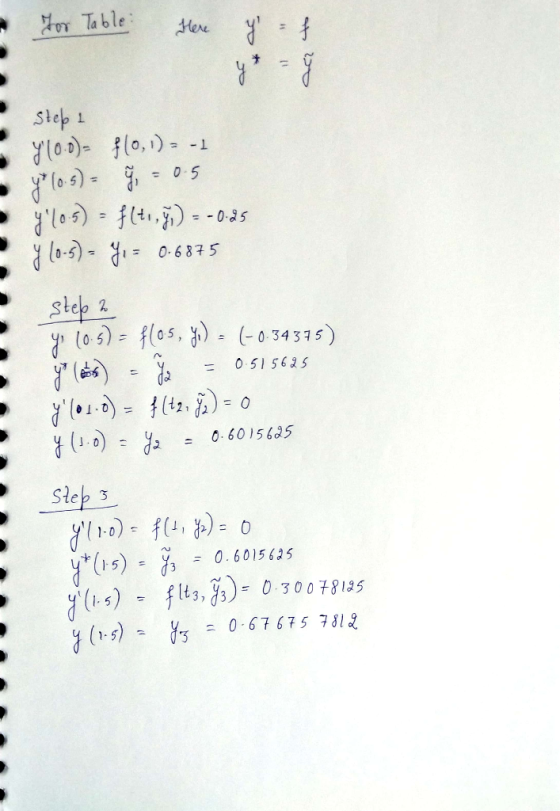
Given the ODE and initial condition 3. y(0) = 1 dt=yi-y Use the explicit predictor-corrector (Heun's)...
For the IVP: Apply Euler-trapezoidal predictor-corrector method to the IVP to approximate y(2), by choosing two...
 For the IVP:
Apply Euler-trapezoidal predictor-corrector method to the IVP to
approximate y(2), by choosing two values of h, for which the
iteration converges. (Note: True Solution: y(t) = et − t
− 1). Present your results in tabular form. Your tabulated results
must contain the exact value, approximate value by the
Euler-trapezoidal predictor-corrector method at t0 = 0,
t1 = 0.5, t2 = 1, t3 = 1.5,
t4 = 2, t5 = 2.5, t6 = 3,
t7 = 3.5...
For the IVP:
Apply Euler-trapezoidal predictor-corrector method to the IVP to
approximate y(2), by choosing two values of h, for which the
iteration converges. (Note: True Solution: y(t) = et − t
− 1). Present your results in tabular form. Your tabulated results
must contain the exact value, approximate value by the
Euler-trapezoidal predictor-corrector method at t0 = 0,
t1 = 0.5, t2 = 1, t3 = 1.5,
t4 = 2, t5 = 2.5, t6 = 3,
t7 = 3.5...
Apply Euler-trapezoidal predictor-corrector method to the IVP in problem 1 to approximate y(2), by choosing two...
 Apply Euler-trapezoidal predictor-corrector method to the IVP in
problem 1 to approximate y(2), by choosing two values of h, for
which the iteration converges. (Don't really need to show work or
do by hand, MATLAB code will work just as well).
1. For the IVP: y' =ty, y(0) = ) 0t 4 Compare the true solution with the approximate solutions from t = 0 to t 4, with the step size h 0.5, obtained by each of the following methods....
Apply Euler-trapezoidal predictor-corrector method to the IVP in
problem 1 to approximate y(2), by choosing two values of h, for
which the iteration converges. (Don't really need to show work or
do by hand, MATLAB code will work just as well).
1. For the IVP: y' =ty, y(0) = ) 0t 4 Compare the true solution with the approximate solutions from t = 0 to t 4, with the step size h 0.5, obtained by each of the following methods....
MATLAB help please!!!!! 1. Use the forward Euler method Vi+,-Vi + (ti+1-tinti , yi) for i=0.1, 2, , taking yo-y(to) to be the initial condition, to approximate the solution at 2 of the IVP y'=y-t...
 MATLAB help please!!!!!
1. Use the forward Euler method Vi+,-Vi + (ti+1-tinti , yi) for i=0.1, 2, , taking yo-y(to) to be the initial condition, to approximate the solution at 2 of the IVP y'=y-t2 + 1, 0 2, y(0) = 0.5. t Use N 2k, k2,...,20 equispaced timesteps so to 0 and t-1 2) Make a convergence plot computing the error by comparing with the exact solution, y: t (t+1)2 exp(t)/2, and plotting the error as a function of...
MATLAB help please!!!!!
1. Use the forward Euler method Vi+,-Vi + (ti+1-tinti , yi) for i=0.1, 2, , taking yo-y(to) to be the initial condition, to approximate the solution at 2 of the IVP y'=y-t2 + 1, 0 2, y(0) = 0.5. t Use N 2k, k2,...,20 equispaced timesteps so to 0 and t-1 2) Make a convergence plot computing the error by comparing with the exact solution, y: t (t+1)2 exp(t)/2, and plotting the error as a function of...
Numerical Methods Consider the following IVP dy=0.01(70-y)(50-y), with y(0)-0 (a) [10 marks Use the Runge-Kutta method of order four to obtain an approximate solution to the ODE at the points t-0.5 an...
 Numerical Methods
Consider the following IVP dy=0.01(70-y)(50-y), with y(0)-0 (a) [10 marks Use the Runge-Kutta method of order four to obtain an approximate solution to the ODE at the points t-0.5 and t1 with a step sizeh 0.5. b) [8 marks Find the exact solution analytically. (c) 7 marks] Use MATLAB to plot the graph of the true and approximate solutions in one figure over the interval [.201. Display graphically the true errors after each steps of calculations.
Consider the...
Numerical Methods
Consider the following IVP dy=0.01(70-y)(50-y), with y(0)-0 (a) [10 marks Use the Runge-Kutta method of order four to obtain an approximate solution to the ODE at the points t-0.5 and t1 with a step sizeh 0.5. b) [8 marks Find the exact solution analytically. (c) 7 marks] Use MATLAB to plot the graph of the true and approximate solutions in one figure over the interval [.201. Display graphically the true errors after each steps of calculations.
Consider the...
Runge-Kutta method R-K method is given by the following algorithm. o y(xo)- given k2-f(xi5.yi tk,...
 Runge-Kutta method R-K method is given by the following algorithm. Yo = y(xo) = given. k1-f(xy) k4-f(xi +h,yi + k3) 6 For i = 0, 1, 2, , n, where h = (b-a)/n. Consider the same IVP given in problem 2 and answer the following a) Write a MATLAB script file to find y(2) using h = 0.1 and call the file odeRK 19.m b) Generate the following table now using both ode Euler and odeRK19 only for h -0.01....
Problem 3. Given the initial conditions, y(0) from t- 0 to 4: and y (0 0, solve the following initial-value problem...
 Problem 3. Given the initial conditions, y(0) from t- 0 to 4: and y (0 0, solve the following initial-value problem d2 dt Obtain your solution with (a) Euler's method and (b) the fourth-order RK method. In both cases, use a step size of 0.1. Plot both solutions on the same graph along with the exact solution y- cos(3t). Note: show the hand calculations for t-0.1 and 0.2, for remaining work use the MATLAB files provided in the lectures
Problem...
Problem 3. Given the initial conditions, y(0) from t- 0 to 4: and y (0 0, solve the following initial-value problem d2 dt Obtain your solution with (a) Euler's method and (b) the fourth-order RK method. In both cases, use a step size of 0.1. Plot both solutions on the same graph along with the exact solution y- cos(3t). Note: show the hand calculations for t-0.1 and 0.2, for remaining work use the MATLAB files provided in the lectures
Problem...
Problem Thre: 125 points) Consider the following initial value problem: dy-2y+ t The y(0) -1 ea dt ical solution of the differential equation is: y(O)(2-2t+3e-2+1)y fr exoc the differential equat...
 Problem Thre: 125 points) Consider the following initial value problem: dy-2y+ t The y(0) -1 ea dt ical solution of the differential equation is: y(O)(2-2t+3e-2+1)y fr exoc the differential equation numerically over the interval 0 s i s 2.0 and a step size h At 0.5.A Apply the following Runge-Kutta methods for each of the step. (show your calculations) i. [0.0 0.5: Euler method ii. [0.5 1.0]: Heun method. ii. [1.0 1.5): Midpoint method. iv. [1.5 2.0): 4h RK method...
Solve using Matlab Use the forward Euler method, Vi+,-Vi+(4+1-tinti ,Vi) for i= 0,1,2, , taking yo y(to) to be the initial condition, to approximate the solution at t-2 of the IVP y'=y-t2 + 1, 0-...
 Solve using Matlab
Use the forward Euler method, Vi+,-Vi+(4+1-tinti ,Vi) for i= 0,1,2, , taking yo y(to) to be the initial condition, to approximate the solution at t-2 of the IVP y'=y-t2 + 1, 0-t-2, y(0) = 0.5. Use N = 2k, k = 1, 2, , 20 equispaced time steps (so to = 0 and tN-1 = 2). Make a convergence plot, computing the error by comparing with the exact solution, y: t1)2 -exp(t)/2, and plotting the error as...
Solve using Matlab
Use the forward Euler method, Vi+,-Vi+(4+1-tinti ,Vi) for i= 0,1,2, , taking yo y(to) to be the initial condition, to approximate the solution at t-2 of the IVP y'=y-t2 + 1, 0-t-2, y(0) = 0.5. Use N = 2k, k = 1, 2, , 20 equispaced time steps (so to = 0 and tN-1 = 2). Make a convergence plot, computing the error by comparing with the exact solution, y: t1)2 -exp(t)/2, and plotting the error as...
Consider the following initial value problem: 1. Use Euler's explicit scheme to solve the above initial value probl...
Consider the following initial value problem: 1. Use Euler's explicit scheme to solve the above initial value problem with time step h= 0.5. Express all the computed results with a precision of three decimal places. 2. The analytical or exact solution is compute the absolute error at each tivalue. Express all the computed results with a precision of three decimal places. 3. Write a matlab function that solves the above (IVP) using (RK2.M) for arbitrary time-step h. y(t) ly(0) 3...
solve it with matlab 25.24 Given the initial conditions, y(0) = 1 and y'(0) = 1...
 solve it with matlab
25.24 Given the initial conditions, y(0) = 1 and y'(0) = 1 and y'(0) = 0, solve the following initial-value problem from t = 0 to 4: dy + 4y = 0 dt² Obtain your solutions with (a) Euler's method and (b) the fourth- order RK method. In both cases, use a step size of 0.125. Plot both solutions on the same graph along with the exact solution y = cos 2t.
solve it with matlab
25.24 Given the initial conditions, y(0) = 1 and y'(0) = 1 and y'(0) = 0, solve the following initial-value problem from t = 0 to 4: dy + 4y = 0 dt² Obtain your solutions with (a) Euler's method and (b) the fourth- order RK method. In both cases, use a step size of 0.125. Plot both solutions on the same graph along with the exact solution y = cos 2t.
 For the IVP:
Apply Euler-trapezoidal predictor-corrector method to the IVP to
approximate y(2), by choosing two values of h, for which the
iteration converges. (Note: True Solution: y(t) = et − t
− 1). Present your results in tabular form. Your tabulated results
must contain the exact value, approximate value by the
Euler-trapezoidal predictor-corrector method at t0 = 0,
t1 = 0.5, t2 = 1, t3 = 1.5,
t4 = 2, t5 = 2.5, t6 = 3,
t7 = 3.5...
For the IVP:
Apply Euler-trapezoidal predictor-corrector method to the IVP to
approximate y(2), by choosing two values of h, for which the
iteration converges. (Note: True Solution: y(t) = et − t
− 1). Present your results in tabular form. Your tabulated results
must contain the exact value, approximate value by the
Euler-trapezoidal predictor-corrector method at t0 = 0,
t1 = 0.5, t2 = 1, t3 = 1.5,
t4 = 2, t5 = 2.5, t6 = 3,
t7 = 3.5...
 Apply Euler-trapezoidal predictor-corrector method to the IVP in
problem 1 to approximate y(2), by choosing two values of h, for
which the iteration converges. (Don't really need to show work or
do by hand, MATLAB code will work just as well).
1. For the IVP: y' =ty, y(0) = ) 0t 4 Compare the true solution with the approximate solutions from t = 0 to t 4, with the step size h 0.5, obtained by each of the following methods....
Apply Euler-trapezoidal predictor-corrector method to the IVP in
problem 1 to approximate y(2), by choosing two values of h, for
which the iteration converges. (Don't really need to show work or
do by hand, MATLAB code will work just as well).
1. For the IVP: y' =ty, y(0) = ) 0t 4 Compare the true solution with the approximate solutions from t = 0 to t 4, with the step size h 0.5, obtained by each of the following methods....
 MATLAB help please!!!!!
1. Use the forward Euler method Vi+,-Vi + (ti+1-tinti , yi) for i=0.1, 2, , taking yo-y(to) to be the initial condition, to approximate the solution at 2 of the IVP y'=y-t2 + 1, 0 2, y(0) = 0.5. t Use N 2k, k2,...,20 equispaced timesteps so to 0 and t-1 2) Make a convergence plot computing the error by comparing with the exact solution, y: t (t+1)2 exp(t)/2, and plotting the error as a function of...
MATLAB help please!!!!!
1. Use the forward Euler method Vi+,-Vi + (ti+1-tinti , yi) for i=0.1, 2, , taking yo-y(to) to be the initial condition, to approximate the solution at 2 of the IVP y'=y-t2 + 1, 0 2, y(0) = 0.5. t Use N 2k, k2,...,20 equispaced timesteps so to 0 and t-1 2) Make a convergence plot computing the error by comparing with the exact solution, y: t (t+1)2 exp(t)/2, and plotting the error as a function of...
 Numerical Methods
Consider the following IVP dy=0.01(70-y)(50-y), with y(0)-0 (a) [10 marks Use the Runge-Kutta method of order four to obtain an approximate solution to the ODE at the points t-0.5 and t1 with a step sizeh 0.5. b) [8 marks Find the exact solution analytically. (c) 7 marks] Use MATLAB to plot the graph of the true and approximate solutions in one figure over the interval [.201. Display graphically the true errors after each steps of calculations.
Consider the...
Numerical Methods
Consider the following IVP dy=0.01(70-y)(50-y), with y(0)-0 (a) [10 marks Use the Runge-Kutta method of order four to obtain an approximate solution to the ODE at the points t-0.5 and t1 with a step sizeh 0.5. b) [8 marks Find the exact solution analytically. (c) 7 marks] Use MATLAB to plot the graph of the true and approximate solutions in one figure over the interval [.201. Display graphically the true errors after each steps of calculations.
Consider the...
 Runge-Kutta method R-K method is given by the following algorithm. Yo = y(xo) = given. k1-f(xy) k4-f(xi +h,yi + k3) 6 For i = 0, 1, 2, , n, where h = (b-a)/n. Consider the same IVP given in problem 2 and answer the following a) Write a MATLAB script file to find y(2) using h = 0.1 and call the file odeRK 19.m b) Generate the following table now using both ode Euler and odeRK19 only for h -0.01....
 Problem 3. Given the initial conditions, y(0) from t- 0 to 4: and y (0 0, solve the following initial-value problem d2 dt Obtain your solution with (a) Euler's method and (b) the fourth-order RK method. In both cases, use a step size of 0.1. Plot both solutions on the same graph along with the exact solution y- cos(3t). Note: show the hand calculations for t-0.1 and 0.2, for remaining work use the MATLAB files provided in the lectures
Problem...
Problem 3. Given the initial conditions, y(0) from t- 0 to 4: and y (0 0, solve the following initial-value problem d2 dt Obtain your solution with (a) Euler's method and (b) the fourth-order RK method. In both cases, use a step size of 0.1. Plot both solutions on the same graph along with the exact solution y- cos(3t). Note: show the hand calculations for t-0.1 and 0.2, for remaining work use the MATLAB files provided in the lectures
Problem...
 Problem Thre: 125 points) Consider the following initial value problem: dy-2y+ t The y(0) -1 ea dt ical solution of the differential equation is: y(O)(2-2t+3e-2+1)y fr exoc the differential equation numerically over the interval 0 s i s 2.0 and a step size h At 0.5.A Apply the following Runge-Kutta methods for each of the step. (show your calculations) i. [0.0 0.5: Euler method ii. [0.5 1.0]: Heun method. ii. [1.0 1.5): Midpoint method. iv. [1.5 2.0): 4h RK method...
 Solve using Matlab
Use the forward Euler method, Vi+,-Vi+(4+1-tinti ,Vi) for i= 0,1,2, , taking yo y(to) to be the initial condition, to approximate the solution at t-2 of the IVP y'=y-t2 + 1, 0-t-2, y(0) = 0.5. Use N = 2k, k = 1, 2, , 20 equispaced time steps (so to = 0 and tN-1 = 2). Make a convergence plot, computing the error by comparing with the exact solution, y: t1)2 -exp(t)/2, and plotting the error as...
Solve using Matlab
Use the forward Euler method, Vi+,-Vi+(4+1-tinti ,Vi) for i= 0,1,2, , taking yo y(to) to be the initial condition, to approximate the solution at t-2 of the IVP y'=y-t2 + 1, 0-t-2, y(0) = 0.5. Use N = 2k, k = 1, 2, , 20 equispaced time steps (so to = 0 and tN-1 = 2). Make a convergence plot, computing the error by comparing with the exact solution, y: t1)2 -exp(t)/2, and plotting the error as...
 solve it with matlab
25.24 Given the initial conditions, y(0) = 1 and y'(0) = 1 and y'(0) = 0, solve the following initial-value problem from t = 0 to 4: dy + 4y = 0 dt² Obtain your solutions with (a) Euler's method and (b) the fourth- order RK method. In both cases, use a step size of 0.125. Plot both solutions on the same graph along with the exact solution y = cos 2t.
solve it with matlab
25.24 Given the initial conditions, y(0) = 1 and y'(0) = 1 and y'(0) = 0, solve the following initial-value problem from t = 0 to 4: dy + 4y = 0 dt² Obtain your solutions with (a) Euler's method and (b) the fourth- order RK method. In both cases, use a step size of 0.125. Plot both solutions on the same graph along with the exact solution y = cos 2t.
Most questions answered within 3 hours.
-
Where is the error in this code sequence?
String s1 = "Hello";
String s2 = "ello";...
asked 11 months ago -
Financial data for Joel de Paris, Inc., for last year
follow:
Joel de Paris, Inc.
Balance...
asked 11 months ago -
Consider this reaction:
Al2(SO4)3 (aq)+ BaCl3
(aq) Al2Cl6 (aq)- +
3BaSO4(s) . What is the...
asked 11 months ago -
Suppose that Savneet is considering increasing her
recent random sample from 20 car rentals to 40...
asked 11 months ago -
Trucks arrive at an unloading terminal at an average rate of 120
per hour.
Trucks arrive...
asked 11 months ago -
Why are methanol and ethanol completely soluble in water while
octanol is not very little soluble....
asked 11 months ago -
A facilities manager at a university reads in a research report
that the mean amount of...
asked 11 months ago -
When the CuSO4 is rehydrated by adding water to the anhydrous
compound, is this an endothermic...
asked 11 months ago -
A ray of sunlight is passing from diamond into crown glass; the
angle of incidence is...
asked 11 months ago -
A block of mass 0.249 kg is placed on top of a light, vertical
spring of...
asked 11 months ago -
how do the kidneys compensate in the presences of acidosis
a) trigger hyperventilate
b) reserve acid...
asked 11 months ago -
Question 501 pts
The rental rate of capital to the firm increases. Which of the
following...
asked 11 months ago