
Homework Answers

To find and plot the Pole Zero Map
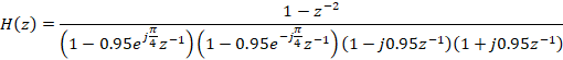
The zeros are at locations where the numerator polynomial is zero. So


So the zeros are at

The poles are at locations where the denominator polynomial is zero. So

First Pole


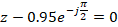
Another way to find the pole is

So the pole is at

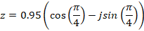
The pole is at the point at an angle
 at a distance
0.95.
at a distance
0.95.
Second Pole


Another way to find the pole is

So the pole is at

The pole is at the point at an angle
 at a distance
0.95.
at a distance
0.95.
Third Pole


Another way to find the pole is

So the pole is at

The pole is at the point at an angle
 at a distance
0.95.
at a distance
0.95.
Fourth Pole


Another way to find the pole is

So the pole is at

The pole is at the point at an angle
 at a distance
0.95.
at a distance
0.95.
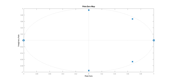
So the poles are at

Hence the pole zero plot will be
To find and plot the Magnitude Response

We know that


So

Using

We get


To get the frequency response put


Using MATLAB
clc;
clear all;
close all;
b = [1, 0, -1];
a1 = [1, -1.3435, 0.9025];
a2 = [1, 0, 0.9025];
a = conv(a1, a2);
w = -pi:pi/1000:pi;
H = freqz(b, a, w);
plot(w/pi, abs(H), 'linewidth', 2);
grid;
xlabel('Normalized Frequency, \omega (\times \pi units)');
ylabel('|H(e^{j\omega})|');
title('Magnitude Response');
sys = tf(b,a,1)
figure
pzmap(sys)
After executing we get

Add Answer to:
please show steps and formulas.
Plot the magnitude of the and the pole- zero plot frequency...
2. Consider a second IIR filter a. Determine the system function H(z), pole-zero location (patterns), and plot the pole-zero pattern. b. Determine the analytical expression for frequency response...
 2. Consider a second IIR filter a. Determine the system function H(z), pole-zero location (patterns), and plot the pole-zero pattern. b. Determine the analytical expression for frequency response, magnitude, and phase response. c. Choose b so that the maximum magnitude response is equal to 1. d. Plot the pole-zero pattern and the magnitude of the frequency response as a function of normal frequency.
2. Consider a second IIR filter a. Determine the system function H(z), pole-zero location (patterns), and plot...
2. Consider a second IIR filter a. Determine the system function H(z), pole-zero location (patterns), and plot the pole-zero pattern. b. Determine the analytical expression for frequency response, magnitude, and phase response. c. Choose b so that the maximum magnitude response is equal to 1. d. Plot the pole-zero pattern and the magnitude of the frequency response as a function of normal frequency.
2. Consider a second IIR filter a. Determine the system function H(z), pole-zero location (patterns), and plot...
For each of the transfer functions given below, draw the pole-zero plot and plot the magnitude separate from the phase as a function of frequency. Show only the asymptotic terms that make up the tra...
 For each of the transfer functions given below, draw the pole-zero plot and plot the magnitude separate from the phase as a function of frequency. Show only the asymptotic terms that make up the transfer function and then add them to show the composite plot. You can verify your plots (to some extent) by using MATLAB to generate the plots but only as a check that the work you have done is correct. The work that will count for points...
5) Design a one-pole, one-zero passive filter to have a low-frequency gain of -32 dB, a high-freq...
 please show all steps and matlab plot ,
5) Design a one-pole, one-zero passive filter to have a low-frequency gain of -32 dB, a high-frequency gain of 0 dB, and a cutoff frequency of 2,000 Hz. Specify the circuit and all component values. Use Matlab to plot the magnitude and phase frequency response for your filter.
5) Design a one-pole, one-zero passive filter to have a low-frequency gain of -32 dB, a high-frequency gain of 0 dB, and a cutoff...
please show all steps and matlab plot ,
5) Design a one-pole, one-zero passive filter to have a low-frequency gain of -32 dB, a high-frequency gain of 0 dB, and a cutoff frequency of 2,000 Hz. Specify the circuit and all component values. Use Matlab to plot the magnitude and phase frequency response for your filter.
5) Design a one-pole, one-zero passive filter to have a low-frequency gain of -32 dB, a high-frequency gain of 0 dB, and a cutoff...
I (K Pole-Zero Plot #1 Pole-Eero Plot 15 L. Pole-Zero Plot IMI 4z1 15 Prde-Zero Plot...
 I (K Pole-Zero Plot #1 Pole-Eero Plot 15 L. Pole-Zero Plot IMI 4z1 15 Prde-Zero Plot #5 Pole-Zero Plat #6 Tine Index (n) Problem P-10.20. Match a pole-zero plot (1-6) to each of the impulse response plots (J-N) shown above (Figure P-10.20 from p. 464) Note: Beach Board causes the magnitude Impulse Response Plot number order to be in random order Pole-Zero Plot #1 Pole-Zero Plot #2 Pole-Zero Plot #3 1, hin] Plot (N) hin] Plot (K) h[n] Plot (M)...
Below is the zero and poles plot of a system. What is the magnitude response of this system? Pole...
 Below is the zero and poles plot of a system. What is the magnitude response of this system? Pole/Zero Plot 0.5 0 0.5 0.5 0 Real Part 0.5 H(J) : (exp(2*90i*theta)-2"exp(%itthet exp(2-i.6)-2 exp(i-0)+2 exp(2 i.)-exp(i.0)+0.5 Your last answer was interpreted as follows: CHR The variables found in your answer were: [e] Incorrect answer.
Below is the zero and poles plot of a system. What is the magnitude response of this system? Pole/Zero Plot 0.5 0 0.5 0.5 0 Real Part...
Below is the zero and poles plot of a system. What is the magnitude response of this system? Pole/Zero Plot 0.5 0 0.5 0.5 0 Real Part 0.5 H(J) : (exp(2*90i*theta)-2"exp(%itthet exp(2-i.6)-2 exp(i-0)+2 exp(2 i.)-exp(i.0)+0.5 Your last answer was interpreted as follows: CHR The variables found in your answer were: [e] Incorrect answer.
Below is the zero and poles plot of a system. What is the magnitude response of this system? Pole/Zero Plot 0.5 0 0.5 0.5 0 Real Part...
no need for pole-zero plot 7. Determine the system function, magnitude response, and phase response of...
 no need for pole-zero plot
7. Determine the system function, magnitude response, and phase response of the fol- lowing systems and use the pole-zero pattern to explain the shape of their magnitude response (a) y[n] = 1(x(n]-x(n-1), ln -2
no need for pole-zero plot
7. Determine the system function, magnitude response, and phase response of the fol- lowing systems and use the pole-zero pattern to explain the shape of their magnitude response (a) y[n] = 1(x(n]-x(n-1), ln -2
For each of the transfer functions given below, draw the pole-zero plot and using the log- semilog paper provided on Blackboard to plot the magnitude separate from the phase as a function of frequenc...
 For each of the transfer functions given below, draw the pole-zero plot and using the log- semilog paper provided on Blackboard to plot the magnitude separate from the phase as a function of frequency. Show only the asymptotic terms that make up the transfer function and then add them to show the composite plot. You can verify your plots (to some extent) by using MATLAB to generate the plots but only as a check that the work you have done...
Problem 4 Questions about the frequency response of an FIR filter: (a) Determine a formula for th...
 Please show all work
Problem 4 Questions about the frequency response of an FIR filter: (a) Determine a formula for the frequency response of an FIR filter defined by the pole-zero plot below: Pole-Zero Plot #1 0.5 -0.5 -1 1 -0.5 0 051 Real part (b) For the FIR filter in part (a), write a simplified version of the frequency response H(e'ω) and use it to prove that the maximum value of the frequency response magnitude will be at ω-tr/2....
Please show all work
Problem 4 Questions about the frequency response of an FIR filter: (a) Determine a formula for the frequency response of an FIR filter defined by the pole-zero plot below: Pole-Zero Plot #1 0.5 -0.5 -1 1 -0.5 0 051 Real part (b) For the FIR filter in part (a), write a simplified version of the frequency response H(e'ω) and use it to prove that the maximum value of the frequency response magnitude will be at ω-tr/2....
The pole-zero plot of a cosine oscillator filter is shown below. The oscillation frequency is one...
 The pole-zero plot of a cosine oscillator filter is shown below. The oscillation frequency is one quarter of the sampling frequency (Fs/4). Pole-Zero Plot for the Non-Damped Cosine Oscillator zp R-1 0.8 06 0.4 0.2 zct zc2 2nd order -0.2 -0.4 -0.6 -0.8 -1 zp -1 -0.5 0.5 Real Part O True False Imaginary Part
Question 3 The pole-zero plot of a sinusoidal oscillator filter is shown below. If the system...
 Question 3 The pole-zero plot of a sinusoidal oscillator filter is shown below. If the system is working at Fs = 8000Hz, the output tone has a frequency of 1000 Hz. Pole-Zero Plot for the Non-Damped Cosine Oscillator Imaginary Part 201 202 2nd order The X zp -1 -0. 50 0. 51 Real Part True False
 2. Consider a second IIR filter a. Determine the system function H(z), pole-zero location (patterns), and plot the pole-zero pattern. b. Determine the analytical expression for frequency response, magnitude, and phase response. c. Choose b so that the maximum magnitude response is equal to 1. d. Plot the pole-zero pattern and the magnitude of the frequency response as a function of normal frequency.
2. Consider a second IIR filter a. Determine the system function H(z), pole-zero location (patterns), and plot...
2. Consider a second IIR filter a. Determine the system function H(z), pole-zero location (patterns), and plot the pole-zero pattern. b. Determine the analytical expression for frequency response, magnitude, and phase response. c. Choose b so that the maximum magnitude response is equal to 1. d. Plot the pole-zero pattern and the magnitude of the frequency response as a function of normal frequency.
2. Consider a second IIR filter a. Determine the system function H(z), pole-zero location (patterns), and plot...
 For each of the transfer functions given below, draw the pole-zero plot and plot the magnitude separate from the phase as a function of frequency. Show only the asymptotic terms that make up the transfer function and then add them to show the composite plot. You can verify your plots (to some extent) by using MATLAB to generate the plots but only as a check that the work you have done is correct. The work that will count for points...
 please show all steps and matlab plot ,
5) Design a one-pole, one-zero passive filter to have a low-frequency gain of -32 dB, a high-frequency gain of 0 dB, and a cutoff frequency of 2,000 Hz. Specify the circuit and all component values. Use Matlab to plot the magnitude and phase frequency response for your filter.
5) Design a one-pole, one-zero passive filter to have a low-frequency gain of -32 dB, a high-frequency gain of 0 dB, and a cutoff...
please show all steps and matlab plot ,
5) Design a one-pole, one-zero passive filter to have a low-frequency gain of -32 dB, a high-frequency gain of 0 dB, and a cutoff frequency of 2,000 Hz. Specify the circuit and all component values. Use Matlab to plot the magnitude and phase frequency response for your filter.
5) Design a one-pole, one-zero passive filter to have a low-frequency gain of -32 dB, a high-frequency gain of 0 dB, and a cutoff...
 I (K Pole-Zero Plot #1 Pole-Eero Plot 15 L. Pole-Zero Plot IMI 4z1 15 Prde-Zero Plot #5 Pole-Zero Plat #6 Tine Index (n) Problem P-10.20. Match a pole-zero plot (1-6) to each of the impulse response plots (J-N) shown above (Figure P-10.20 from p. 464) Note: Beach Board causes the magnitude Impulse Response Plot number order to be in random order Pole-Zero Plot #1 Pole-Zero Plot #2 Pole-Zero Plot #3 1, hin] Plot (N) hin] Plot (K) h[n] Plot (M)...
 Below is the zero and poles plot of a system. What is the magnitude response of this system? Pole/Zero Plot 0.5 0 0.5 0.5 0 Real Part 0.5 H(J) : (exp(2*90i*theta)-2"exp(%itthet exp(2-i.6)-2 exp(i-0)+2 exp(2 i.)-exp(i.0)+0.5 Your last answer was interpreted as follows: CHR The variables found in your answer were: [e] Incorrect answer.
Below is the zero and poles plot of a system. What is the magnitude response of this system? Pole/Zero Plot 0.5 0 0.5 0.5 0 Real Part...
Below is the zero and poles plot of a system. What is the magnitude response of this system? Pole/Zero Plot 0.5 0 0.5 0.5 0 Real Part 0.5 H(J) : (exp(2*90i*theta)-2"exp(%itthet exp(2-i.6)-2 exp(i-0)+2 exp(2 i.)-exp(i.0)+0.5 Your last answer was interpreted as follows: CHR The variables found in your answer were: [e] Incorrect answer.
Below is the zero and poles plot of a system. What is the magnitude response of this system? Pole/Zero Plot 0.5 0 0.5 0.5 0 Real Part...
 no need for pole-zero plot
7. Determine the system function, magnitude response, and phase response of the fol- lowing systems and use the pole-zero pattern to explain the shape of their magnitude response (a) y[n] = 1(x(n]-x(n-1), ln -2
no need for pole-zero plot
7. Determine the system function, magnitude response, and phase response of the fol- lowing systems and use the pole-zero pattern to explain the shape of their magnitude response (a) y[n] = 1(x(n]-x(n-1), ln -2
 For each of the transfer functions given below, draw the pole-zero plot and using the log- semilog paper provided on Blackboard to plot the magnitude separate from the phase as a function of frequency. Show only the asymptotic terms that make up the transfer function and then add them to show the composite plot. You can verify your plots (to some extent) by using MATLAB to generate the plots but only as a check that the work you have done...
 Please show all work
Problem 4 Questions about the frequency response of an FIR filter: (a) Determine a formula for the frequency response of an FIR filter defined by the pole-zero plot below: Pole-Zero Plot #1 0.5 -0.5 -1 1 -0.5 0 051 Real part (b) For the FIR filter in part (a), write a simplified version of the frequency response H(e'ω) and use it to prove that the maximum value of the frequency response magnitude will be at ω-tr/2....
Please show all work
Problem 4 Questions about the frequency response of an FIR filter: (a) Determine a formula for the frequency response of an FIR filter defined by the pole-zero plot below: Pole-Zero Plot #1 0.5 -0.5 -1 1 -0.5 0 051 Real part (b) For the FIR filter in part (a), write a simplified version of the frequency response H(e'ω) and use it to prove that the maximum value of the frequency response magnitude will be at ω-tr/2....
 The pole-zero plot of a cosine oscillator filter is shown below. The oscillation frequency is one quarter of the sampling frequency (Fs/4). Pole-Zero Plot for the Non-Damped Cosine Oscillator zp R-1 0.8 06 0.4 0.2 zct zc2 2nd order -0.2 -0.4 -0.6 -0.8 -1 zp -1 -0.5 0.5 Real Part O True False Imaginary Part
 Question 3 The pole-zero plot of a sinusoidal oscillator filter is shown below. If the system is working at Fs = 8000Hz, the output tone has a frequency of 1000 Hz. Pole-Zero Plot for the Non-Damped Cosine Oscillator Imaginary Part 201 202 2nd order The X zp -1 -0. 50 0. 51 Real Part True False
Most questions answered within 3 hours.
-
Where is the error in this code sequence?
String s1 = "Hello";
String s2 = "ello";...
asked 10 months ago -
Financial data for Joel de Paris, Inc., for last year
follow:
Joel de Paris, Inc.
Balance...
asked 10 months ago -
Consider this reaction:
Al2(SO4)3 (aq)+ BaCl3
(aq) Al2Cl6 (aq)- +
3BaSO4(s) . What is the...
asked 10 months ago -
Suppose that Savneet is considering increasing her
recent random sample from 20 car rentals to 40...
asked 10 months ago -
Trucks arrive at an unloading terminal at an average rate of 120
per hour.
Trucks arrive...
asked 10 months ago -
Why are methanol and ethanol completely soluble in water while
octanol is not very little soluble....
asked 10 months ago -
A facilities manager at a university reads in a research report
that the mean amount of...
asked 10 months ago -
When the CuSO4 is rehydrated by adding water to the anhydrous
compound, is this an endothermic...
asked 10 months ago -
A ray of sunlight is passing from diamond into crown glass; the
angle of incidence is...
asked 10 months ago -
A block of mass 0.249 kg is placed on top of a light, vertical
spring of...
asked 10 months ago -
how do the kidneys compensate in the presences of acidosis
a) trigger hyperventilate
b) reserve acid...
asked 10 months ago -
Question 501 pts
The rental rate of capital to the firm increases. Which of the
following...
asked 10 months ago