

Homework Answers


Code to copy
%Code
1.a
%Given
%Declare and initialize R
R_Val=10;
%Declare and initialize r
r_Val=1.8;
%Declare and initialize d
d_Val=0.8;
%Declare and initialize a
a_Val=0.5;
%Declare and initialize steps
steps = 0.1;
%Declare and initialize t
t_Val=0: steps: 200;
%Compute x
x_Val = (((R_Val-r_Val).*cos(t_Val)) + (d_Val.*
cos(((R_Val-r_Val)./r_Val).*t_Val)));
%Compute y
y_Val = (((R_Val-r_Val).*sin(t_Val)) + (d_Val.*
sin(((R_Val-r_Val)./r_Val).*t_Val))) .* cos(a_Val.*t_Val);
%Compute z
z_Val = (((R_Val-r_Val).*sin(t_Val)) + (d_Val.*
sin(((R_Val-r_Val)./r_Val).*t_Val))) .* sin(a_Val.*t_Val);
%Plot 3D graph
plot3(x_Val, y_Val, z_Val)
%Code
1.b
%Given
%Declare and initialize R
R_Val=10;
%Declare and initialize r
r_Val=1.8;
%Declare and initialize d
d_Val=0.8;
%Declare and initialize a
a_Val=0.5;
%Declare and initialize steps
steps = 0.1;
%Declare and initialize t
t_Val = 0: steps: 40;
%Compute x
x_Val = (((R_Val-r_Val).*cos(t_Val)) + (d_Val.*
cos(((R_Val-r_Val)./r_Val).*t_Val)));
%Compute y
y_Val = (((R_Val-r_Val).*sin(t_Val)) + (d_Val.*
sin(((R_Val-r_Val)./r_Val).*t_Val))) .* cos(a_Val.*t_Val);
%Compute z
z_Val = (((R_Val-r_Val).*sin(t_Val)) + (d_Val.*
sin(((R_Val-r_Val)./r_Val).*t_Val))) .* sin(a_Val.*t_Val);
%Plot 3D graph with yellow color
plot3(x_Val, y_Val, z_Val, 'y')
%Hold
hold on;
%Declare and initialize t
t_Val = 40: steps: 80;
%Compute x
x_Val = (((R_Val-r_Val).*cos(t_Val)) + (d_Val.*
cos(((R_Val-r_Val)./r_Val).*t_Val)));
%Compute y
y_Val = (((R_Val-r_Val).*sin(t_Val)) + (d_Val.*
sin(((R_Val-r_Val)./r_Val).*t_Val))) .* cos(a_Val.*t_Val);
%Compute z
z_Val = (((R_Val-r_Val).*sin(t_Val)) + (d_Val.*
sin(((R_Val-r_Val)./r_Val).*t_Val))) .* sin(a_Val.*t_Val);
%Plot 3D graph with red color
plot3(x_Val, y_Val, z_Val, 'r')
%Hold
hold on;
%Declare and initialize t
t_Val = 80: steps: 120;
%Compute x
x_Val = (((R_Val-r_Val).*cos(t_Val)) + (d_Val.*
cos(((R_Val-r_Val)./r_Val).*t_Val)));
%Compute y
y_Val = (((R_Val-r_Val).*sin(t_Val)) + (d_Val.*
sin(((R_Val-r_Val)./r_Val).*t_Val))) .* cos(a_Val.*t_Val);
%Compute z
z_Val = (((R_Val-r_Val).*sin(t_Val)) + (d_Val.*
sin(((R_Val-r_Val)./r_Val).*t_Val))) .* sin(a_Val.*t_Val);
%Plot 3D graph with green color
plot3(x_Val, y_Val, z_Val, 'g')
%Hold
hold on;
%Declare and initialize t
t_Val = 120: steps: 160;
%Compute x
x_Val = (((R_Val-r_Val).*cos(t_Val)) + (d_Val.*
cos(((R_Val-r_Val)./r_Val).*t_Val)));
%Compute y
y_Val = (((R_Val-r_Val).*sin(t_Val)) + (d_Val.*
sin(((R_Val-r_Val)./r_Val).*t_Val))) .* cos(a_Val.*t_Val);
%Compute z
z_Val = (((R_Val-r_Val).*sin(t_Val)) + (d_Val.*
sin(((R_Val-r_Val)./r_Val).*t_Val))) .* sin(a_Val.*t_Val);
%Plot 3D graph with magenta color
plot3(x_Val, y_Val, z_Val, 'm')
%Hold
hold on;
%Declare and initialize t
t_Val = 160: steps: 200;
%Compute x
x_Val = (((R_Val-r_Val).*cos(t_Val)) + (d_Val.*
cos(((R_Val-r_Val)./r_Val).*t_Val)));
%Compute y
y_Val = (((R_Val-r_Val).*sin(t_Val)) + (d_Val.*
sin(((R_Val-r_Val)./r_Val).*t_Val))) .* cos(a_Val.*t_Val);
%Compute z
z_Val = (((R_Val-r_Val).*sin(t_Val)) + (d_Val.*
sin(((R_Val-r_Val)./r_Val).*t_Val))) .* sin(a_Val.*t_Val);
%Plot 3D graph with blue color
plot3(x_Val, y_Val, z_Val, 'b')
%Hold
hold on;
Add Answer to:
MATLAB
ICA 1: a) Using plot3, plot x, y and z given by the follow equations,...
Using matlab, create a 3-D plot of the wave equation y(x,t)= cos(omega*t-beta*x) .Plot for a time...
Using matlab, create a 3-D plot of the wave equation y(x,t)= cos(omega*t-beta*x) .Plot for a time range from t=0 to t=2T and a space range of x=0 to x=2lambda
Using matlab, write the code and plot the graph for the following equations. The x axis...
 Using matlab, write the code and plot the graph for the
following equations. The x axis would be theta from 0 deg to 360
deg while the y axis would be angular or tangential position,
velocity and acceleration.
10 100 E7360 AB- eD100mm sin 1O-Sn 2To ne cose, t Cas 2 3 4 O,= To (reano,re bease-feo, sene-Feo 6 as ) Cos O2
10 100 E7360 AB- eD100mm sin 1O-Sn 2To ne cose, t Cas 2 3 4 O,= To...
Using matlab, write the code and plot the graph for the
following equations. The x axis would be theta from 0 deg to 360
deg while the y axis would be angular or tangential position,
velocity and acceleration.
10 100 E7360 AB- eD100mm sin 1O-Sn 2To ne cose, t Cas 2 3 4 O,= To (reano,re bease-feo, sene-Feo 6 as ) Cos O2
10 100 E7360 AB- eD100mm sin 1O-Sn 2To ne cose, t Cas 2 3 4 O,= To...
I'm trying to solve this differential equations by using matlab and I've got a plot from the code attached. But...
 I'm
trying to solve this differential equations by using matlab and
I've got a plot from the code attached. But I wanna get a plot of
completely sinusoidal form. If I can magnify the plot and expand
x-axis, maybe we can get the sinusoidal form. So help me with this
problem by using matlab. Example is attached in below. One is the
plot from this code and another is example.
function second_order_ode2
t=[0:0.001:1];
initial_x=0;
initial_dxdt=0;
[t,x]=ode45(@rhs,t,[initial_x initial_dxdt]);
plot(t,x(:,1))
xlabel('t')
ylabel('x')...
I'm
trying to solve this differential equations by using matlab and
I've got a plot from the code attached. But I wanna get a plot of
completely sinusoidal form. If I can magnify the plot and expand
x-axis, maybe we can get the sinusoidal form. So help me with this
problem by using matlab. Example is attached in below. One is the
plot from this code and another is example.
function second_order_ode2
t=[0:0.001:1];
initial_x=0;
initial_dxdt=0;
[t,x]=ode45(@rhs,t,[initial_x initial_dxdt]);
plot(t,x(:,1))
xlabel('t')
ylabel('x')...
(USING MATLAB) Given two differential equations X= sin(t)(exp(cos(t))-2cos(4t)+sin(t/12)^5) And Y = cos(t)(exp(cos(t))-2cos(4t)+sin(t/12)^5) where 0<t<20pi is a...
(USING MATLAB) Given two differential equations X= sin(t)(exp(cos(t))-2cos(4t)+sin(t/12)^5) And Y = cos(t)(exp(cos(t))-2cos(4t)+sin(t/12)^5) where 0<t<20pi is a vector of 5000 points created by using (linspace) command : Write script to plot X and Y with red color ?
I'm trying to solve this differential equations by using matlab and I've got a plot from the code attached. But...
 I'm
trying to solve this differential equations by using matlab and
I've got a plot from the code attached. But I wanna get a plot of
completely sinusoidal form. If I can magnify the plot and expand
x-axis, maybe we can get the sinusoidal form. So help me with this
problem by using matlab. Example is attached in below. One is the
plot from this code and another is example.
function second_order_ode2
t=[0:0.001:1];
initial_x=0;
initial_dxdt=0;
[t,x]=ode45(@rhs,t,[initial_x initial_dxdt]);
plot(t,x(:,1))
xlabel('t')
ylabel('x')...
I'm
trying to solve this differential equations by using matlab and
I've got a plot from the code attached. But I wanna get a plot of
completely sinusoidal form. If I can magnify the plot and expand
x-axis, maybe we can get the sinusoidal form. So help me with this
problem by using matlab. Example is attached in below. One is the
plot from this code and another is example.
function second_order_ode2
t=[0:0.001:1];
initial_x=0;
initial_dxdt=0;
[t,x]=ode45(@rhs,t,[initial_x initial_dxdt]);
plot(t,x(:,1))
xlabel('t')
ylabel('x')...
1. Find general solutions to the following differential systems of equations using dsolve: a. x' =...
 1. Find general solutions to the following differential systems of equations using dsolve: a. x' = y + t, y' = 2 -x+t b. x'=s-X, y' = -y - 3x, C. X" = x - x - y, y = -x- y - y - s', s" = -95 d. Solve the equations in c. above with the initial conditions x(0) = 1, x'(0) = 0, y(0) = -1, y'(0) = 0, $(0) = 1, s'(0) = 0, and plot...
To plot a figure of a function y=f(t) in an interval a and b in MATLAB,...
 To plot a figure of a function y=f(t) in an interval a and b in MATLAB, one should find n-1 points of t between a and b and then find the corresponding values to plot the figure. Below shows an example of a sin function in the range of 0 and 1 with 1000 increments, as well as the figure. >> t = 0:0.001:1; >> y = sin(2*pi*2*t); >> figure >> plot(t, y) 0 02 04 06 08 Demonstrate a...
Match the graphs with their parametric equations. II y 2.0 kor 1.51 0.5 1.01 -1.0 -0.5...
 Match the graphs with their parametric equations. II y 2.0 kor 1.51 0.5 1.01 -1.0 -0.5 0.5 1.0 0.5 -0.51 -1.0 -0.5 0.5 1.0 ho IV 8 III у 0.21 6 0.1 х 40.2 -0.1 0.1 0.2 -0.1 -0.2 VI v у 11.06 у 0 0.B os 0.6 0.4 |-ho -0.5 0.5 102 -0.5 0.5 1.0 1.5 2.0 2.5 3.0 (a) x = 44 - t + 1, y = 42 Х IV = 42 – 2t, y = VE...
Required: MATLAB CODE and attached figure window for the this question. 12. Make the plot of the astroid that is shown...
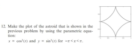 Required: MATLAB CODE and attached figure window for the this
question.
12. Make the plot of the astroid that is shown in the is problem by using the parametric equa- 0.5 tion: 05 0s cos'() and y -sin'(t) for -x<T
12. Make the plot of the astroid that is shown in the is problem by using the parametric equa- 0.5 tion: 05 0s cos'() and y -sin'(t) for -x
Required: MATLAB CODE and attached figure window for the this
question.
12. Make the plot of the astroid that is shown in the is problem by using the parametric equa- 0.5 tion: 05 0s cos'() and y -sin'(t) for -x<T
12. Make the plot of the astroid that is shown in the is problem by using the parametric equa- 0.5 tion: 05 0s cos'() and y -sin'(t) for -x
MATLAB, Please answer question 1. + ENGR 102 Homework 9 :- 1) An elliptical staircase that...
 MATLAB, Please answer question 1.
+ ENGR 102 Homework 9 :- 1) An elliptical staircase that decreases in size with height can be modeled by the parametric equations: r cos(t) y-rsint) it m) Where, e-0.04t Ib cos(O)+ [a sin()]- a and b are the semimajor and semiminor axes of the ellipse, h is the staircase height, and n is the number pf revolutions that the staircase makes. Make a 3-D plot of the staircase with a 20 m, b 10...
MATLAB, Please answer question 1.
+ ENGR 102 Homework 9 :- 1) An elliptical staircase that decreases in size with height can be modeled by the parametric equations: r cos(t) y-rsint) it m) Where, e-0.04t Ib cos(O)+ [a sin()]- a and b are the semimajor and semiminor axes of the ellipse, h is the staircase height, and n is the number pf revolutions that the staircase makes. Make a 3-D plot of the staircase with a 20 m, b 10...
 Using matlab, write the code and plot the graph for the
following equations. The x axis would be theta from 0 deg to 360
deg while the y axis would be angular or tangential position,
velocity and acceleration.
10 100 E7360 AB- eD100mm sin 1O-Sn 2To ne cose, t Cas 2 3 4 O,= To (reano,re bease-feo, sene-Feo 6 as ) Cos O2
10 100 E7360 AB- eD100mm sin 1O-Sn 2To ne cose, t Cas 2 3 4 O,= To...
Using matlab, write the code and plot the graph for the
following equations. The x axis would be theta from 0 deg to 360
deg while the y axis would be angular or tangential position,
velocity and acceleration.
10 100 E7360 AB- eD100mm sin 1O-Sn 2To ne cose, t Cas 2 3 4 O,= To (reano,re bease-feo, sene-Feo 6 as ) Cos O2
10 100 E7360 AB- eD100mm sin 1O-Sn 2To ne cose, t Cas 2 3 4 O,= To...
 I'm
trying to solve this differential equations by using matlab and
I've got a plot from the code attached. But I wanna get a plot of
completely sinusoidal form. If I can magnify the plot and expand
x-axis, maybe we can get the sinusoidal form. So help me with this
problem by using matlab. Example is attached in below. One is the
plot from this code and another is example.
function second_order_ode2
t=[0:0.001:1];
initial_x=0;
initial_dxdt=0;
[t,x]=ode45(@rhs,t,[initial_x initial_dxdt]);
plot(t,x(:,1))
xlabel('t')
ylabel('x')...
I'm
trying to solve this differential equations by using matlab and
I've got a plot from the code attached. But I wanna get a plot of
completely sinusoidal form. If I can magnify the plot and expand
x-axis, maybe we can get the sinusoidal form. So help me with this
problem by using matlab. Example is attached in below. One is the
plot from this code and another is example.
function second_order_ode2
t=[0:0.001:1];
initial_x=0;
initial_dxdt=0;
[t,x]=ode45(@rhs,t,[initial_x initial_dxdt]);
plot(t,x(:,1))
xlabel('t')
ylabel('x')...
 I'm
trying to solve this differential equations by using matlab and
I've got a plot from the code attached. But I wanna get a plot of
completely sinusoidal form. If I can magnify the plot and expand
x-axis, maybe we can get the sinusoidal form. So help me with this
problem by using matlab. Example is attached in below. One is the
plot from this code and another is example.
function second_order_ode2
t=[0:0.001:1];
initial_x=0;
initial_dxdt=0;
[t,x]=ode45(@rhs,t,[initial_x initial_dxdt]);
plot(t,x(:,1))
xlabel('t')
ylabel('x')...
I'm
trying to solve this differential equations by using matlab and
I've got a plot from the code attached. But I wanna get a plot of
completely sinusoidal form. If I can magnify the plot and expand
x-axis, maybe we can get the sinusoidal form. So help me with this
problem by using matlab. Example is attached in below. One is the
plot from this code and another is example.
function second_order_ode2
t=[0:0.001:1];
initial_x=0;
initial_dxdt=0;
[t,x]=ode45(@rhs,t,[initial_x initial_dxdt]);
plot(t,x(:,1))
xlabel('t')
ylabel('x')...
 1. Find general solutions to the following differential systems of equations using dsolve: a. x' = y + t, y' = 2 -x+t b. x'=s-X, y' = -y - 3x, C. X" = x - x - y, y = -x- y - y - s', s" = -95 d. Solve the equations in c. above with the initial conditions x(0) = 1, x'(0) = 0, y(0) = -1, y'(0) = 0, $(0) = 1, s'(0) = 0, and plot...
 To plot a figure of a function y=f(t) in an interval a and b in MATLAB, one should find n-1 points of t between a and b and then find the corresponding values to plot the figure. Below shows an example of a sin function in the range of 0 and 1 with 1000 increments, as well as the figure. >> t = 0:0.001:1; >> y = sin(2*pi*2*t); >> figure >> plot(t, y) 0 02 04 06 08 Demonstrate a...
 Match the graphs with their parametric equations. II y 2.0 kor 1.51 0.5 1.01 -1.0 -0.5 0.5 1.0 0.5 -0.51 -1.0 -0.5 0.5 1.0 ho IV 8 III у 0.21 6 0.1 х 40.2 -0.1 0.1 0.2 -0.1 -0.2 VI v у 11.06 у 0 0.B os 0.6 0.4 |-ho -0.5 0.5 102 -0.5 0.5 1.0 1.5 2.0 2.5 3.0 (a) x = 44 - t + 1, y = 42 Х IV = 42 – 2t, y = VE...
 Required: MATLAB CODE and attached figure window for the this
question.
12. Make the plot of the astroid that is shown in the is problem by using the parametric equa- 0.5 tion: 05 0s cos'() and y -sin'(t) for -x<T
12. Make the plot of the astroid that is shown in the is problem by using the parametric equa- 0.5 tion: 05 0s cos'() and y -sin'(t) for -x
Required: MATLAB CODE and attached figure window for the this
question.
12. Make the plot of the astroid that is shown in the is problem by using the parametric equa- 0.5 tion: 05 0s cos'() and y -sin'(t) for -x<T
12. Make the plot of the astroid that is shown in the is problem by using the parametric equa- 0.5 tion: 05 0s cos'() and y -sin'(t) for -x
 MATLAB, Please answer question 1.
+ ENGR 102 Homework 9 :- 1) An elliptical staircase that decreases in size with height can be modeled by the parametric equations: r cos(t) y-rsint) it m) Where, e-0.04t Ib cos(O)+ [a sin()]- a and b are the semimajor and semiminor axes of the ellipse, h is the staircase height, and n is the number pf revolutions that the staircase makes. Make a 3-D plot of the staircase with a 20 m, b 10...
MATLAB, Please answer question 1.
+ ENGR 102 Homework 9 :- 1) An elliptical staircase that decreases in size with height can be modeled by the parametric equations: r cos(t) y-rsint) it m) Where, e-0.04t Ib cos(O)+ [a sin()]- a and b are the semimajor and semiminor axes of the ellipse, h is the staircase height, and n is the number pf revolutions that the staircase makes. Make a 3-D plot of the staircase with a 20 m, b 10...
Most questions answered within 3 hours.
-
Where is the error in this code sequence?
String s1 = "Hello";
String s2 = "ello";...
asked 11 months ago -
Financial data for Joel de Paris, Inc., for last year
follow:
Joel de Paris, Inc.
Balance...
asked 11 months ago -
Consider this reaction:
Al2(SO4)3 (aq)+ BaCl3
(aq) Al2Cl6 (aq)- +
3BaSO4(s) . What is the...
asked 11 months ago -
Suppose that Savneet is considering increasing her
recent random sample from 20 car rentals to 40...
asked 11 months ago -
Trucks arrive at an unloading terminal at an average rate of 120
per hour.
Trucks arrive...
asked 11 months ago -
Why are methanol and ethanol completely soluble in water while
octanol is not very little soluble....
asked 11 months ago -
A facilities manager at a university reads in a research report
that the mean amount of...
asked 11 months ago -
When the CuSO4 is rehydrated by adding water to the anhydrous
compound, is this an endothermic...
asked 11 months ago -
A ray of sunlight is passing from diamond into crown glass; the
angle of incidence is...
asked 11 months ago -
A block of mass 0.249 kg is placed on top of a light, vertical
spring of...
asked 11 months ago -
how do the kidneys compensate in the presences of acidosis
a) trigger hyperventilate
b) reserve acid...
asked 11 months ago -
Question 501 pts
The rental rate of capital to the firm increases. Which of the
following...
asked 11 months ago