Question

Use Matlab to and the SISOTool construct the system for analysis (You may want to preview the tf and sisotool commands from matlab by typing help tf or doc tf etc...) Each Block B1, B2, B3 and B4 will be constructed individually and then concatenated together As shown in the block diagram let K=0.1 Set B1 = 0.1 by typing in matlab >>B1=0.1 To assign the Blockl values use the TF command to construct a linear time invariant expression on s tf([num coef highest power, ... , coef lowest power ],[den coeft highest power, ..., den coef lowest power]) >> B2=tf([50],[1,0]) >> B3-tf([5],[1,8]) >> B4=tf([15],[1,22]) >> ol=B1*B2*B3*B4 Transfer function: 375 5^3 + 30 s^2 + 176 s You now have the open loop system. Use the sisotool from Matlab to examine the step response and Root Locus >>sisotool(ol) Click to show the step response and delete the Bode Plots

please show work
thank you!

Answer 1

1)MATLAB code used for generating open loop transfer function is

>> k=0.1;
>> g1=tf([100],[1 0])

g1 =

100
---
s

Continuous-time transfer function.

>> g2=tf([2],[1 3])

g2 =

2
-----
s + 3

Continuous-time transfer function.

>> g3=tf([20],[1 30])

g3 =

20
------
s + 30

Continuous-time transfer function.

>> G=k*g1*g2*g3

G =

400
-------------------
s^3 + 33 s^2 + 90 s

Continuous-time transfer function.

>>sisotool(G)

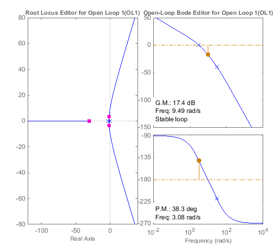
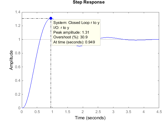
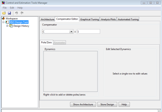
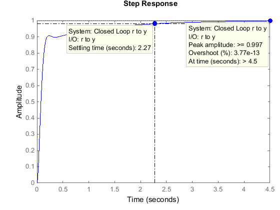
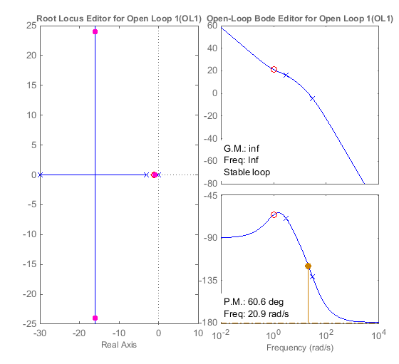
a)Now Gain changed to 0.66 then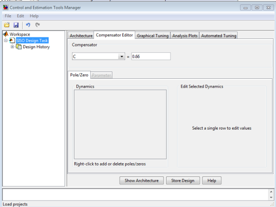

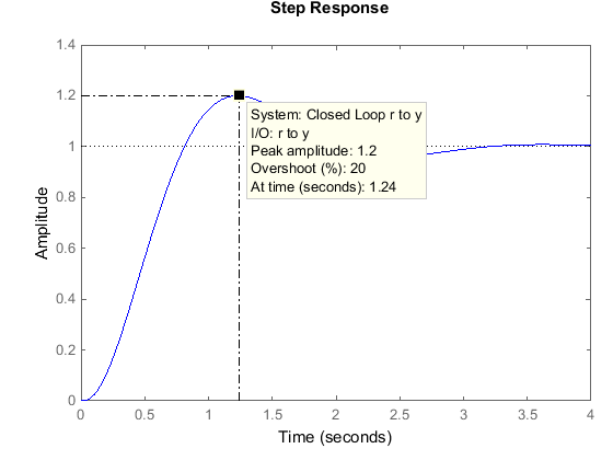
2)zeta =0.707 corresponds 4% overshoot in step response or 65 degree phase margin

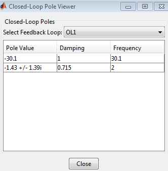
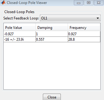
In compensator editor gain choosen as 0.3 then

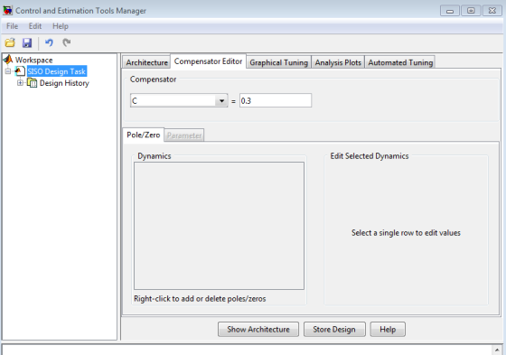
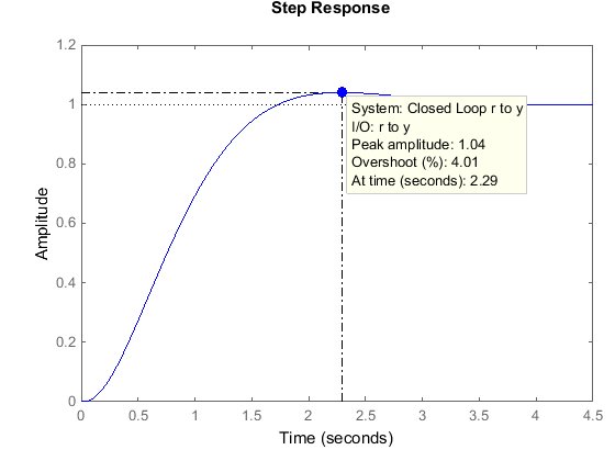
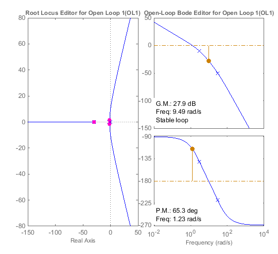
close loop poles are

3)>> figure;rlocus(G)

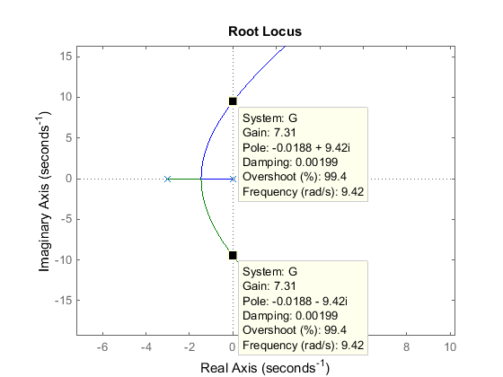
Critical gain becomes 7.3

4)sisotool(G)

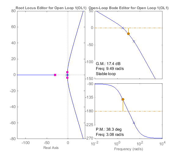
A

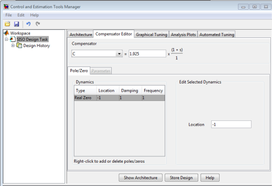
Add zero at s=-1 then

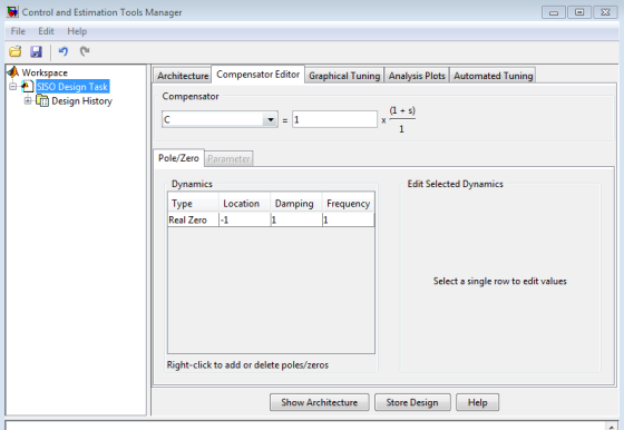
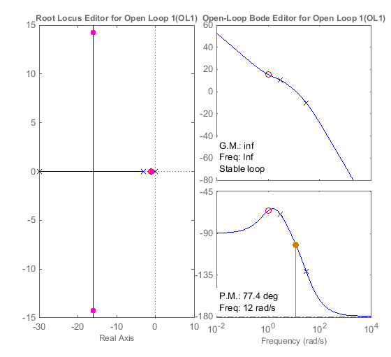
real zero move to the right then root locus moves left side.and settling time reduces i.e transient response improves

Real zero placed at s=1

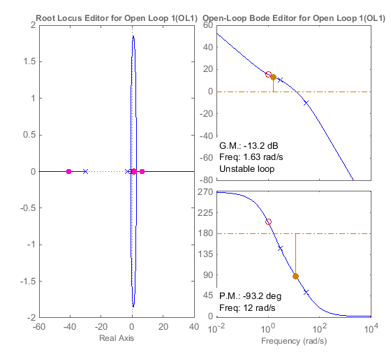
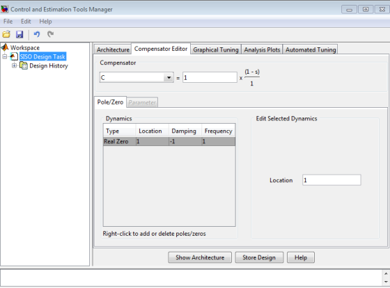
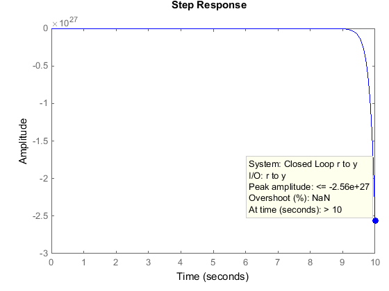
Root locus moves to right side and transient response worsen.

5)real zero located at -1

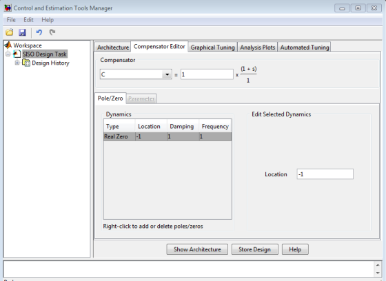
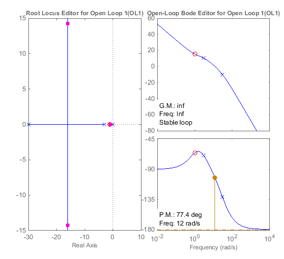
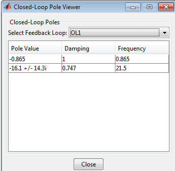
closed loop pole location vary