Question

The following table contains the age of car x1 (in years) and their selling price x2 (in thousands of dollars). x1 3 5 5 7 7 7 8 9 10 11 x2 2.3 1.9 1 0.7 0.3 1 1.05 0.45 0.7 0.4 (a) Compute the generalized distance for each data point. (b) Construct the histogram for marginal variables x1 and x2. Are they normally distributed individually? (c) Construct the appropriate Q-Q plot for the distance data obtained in (a), does (x1, x2) follow a normal distribution jointly? (d) Determine the power transformation for x1 and x2 such that they are marginally normal. (Note: You need to construct the relevant Q-Q plots to demonstrate that the transformed x1 and x2 are normal.)

Answer 1

(a)

x1=c(3, 5, 5, 7, 7, 7, 8, 9, 10, 11)
d1=abs(x1-mean(x1))

4.2 2.2 2.2 0.2 0.2 0.2 0.8 1.8 2.8 3.8

x2=c(2.3, 1.9, 1, 0.7, 0.3, 1, 1.05, 0.45, 0.7, 0.4)
d2=abs(x2-mean(x2))

1.32 0.92 0.02 0.28 0.68 0.02 0.07 0.53 0.28 0.58

(b) We use R command to solve question.

x1=c(3, 5, 5, 7, 7, 7, 8, 9, 10, 11)
x2=c(2.3, 1.9, 1, 0.7, 0.3, 1, 1.05, 0.45, 0.7, 0.4)
par(mfrow=c(1,2))
hist(x1)
hist(x2)

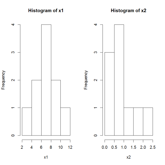
Here, we see from histogram that x1 are normally distributed but x2 is not.

(c)

x1=c(3, 5, 5, 7, 7, 7, 8, 9, 10, 11)
x2=c(2.3, 1.9, 1, 0.7, 0.3, 1, 1.05, 0.45, 0.7, 0.4)
par(mfrow=c(1,2))
qqnorm(x1)
qqline(x1)
qqnorm(x2)
qqline(x2)

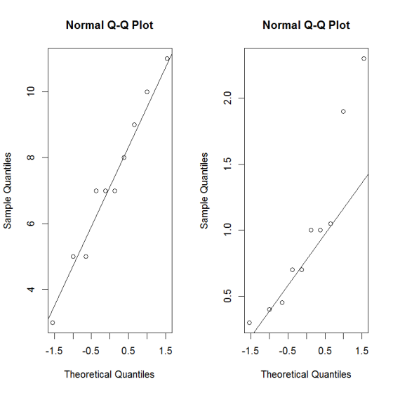
As all the points of x1 fall approximately along this reference line, we can assume normality.

But higher values of x2 is far from the line. So, it is not normal.

(d)

If we taken exponential transformation in x2 variable, then it may be approximate to normal