Question

	Delta	IBM
Jan-83	0.04	0.027
Feb-83	0.027	0.01
Mar-83	-0.016	0.028
Apr-83	-0.043	0.15
May-83	-0.045	-0.041
Jun-83	0.012	0.081
Jul-83	-0.259	0.001
Aug-83	0.08	0.001
Sep-83	0.041	0.062
Oct-83	0.039	-0.001
Nov-83	0.12	-0.066
Dec-83	-0.028	0.039
Jan-84	-0.013	-0.065
Feb-84	-0.117	-0.026
Mar-84	0.065	0.034
Apr-84	-0.085	-0.002
May-84	-0.07	-0.044
Jun-84	-0.012	-0.019
Jul-84	0.045	0.047
Aug-84	0.04	0.127
Sep-84	0.008	0.004
Oct-84	0.161	0.012
Nov-84	-0.026	-0.023
Dec-84	0.156	0.011
Jan-85	-0.01	0.108
Feb-85	0.087	-0.009
Mar-85	-0.003	-0.052
Apr-85	-0.123	-0.004
May-85	0.179	0.025
Jun-85	0.021	-0.038
Jul-85	0.008	0.062
Aug-85	-0.066	-0.028
Sep-85	-0.112	-0.022
Oct-85	-0.083	0.048
Nov-85	0.02	0.085
Dec-85	0.03	0.113
Jan-86	0.122	-0.026
Feb-86	-0.055	0.003
Mar-86	0.076	0.004
Apr-86	0.059	0.031
May-86	-0.043	-0.018
Jun-86	-0.07	-0.039
Jul-86	0.018	-0.096
Aug-86	0.018	0.055
Sep-86	0.026	-0.031
Oct-86	0.134	-0.081
Nov-86	-0.018	0.037
Dec-86	-0.01	-0.056
Jan-87	0.161	0.073
Feb-87	0.133	0.092
Mar-87	-0.129	0.076
Apr-87	-0.121	0.067
May-87	0.151	0.006
Jun-87	0.014	0.016
Jul-87	0.043	-0.009
Aug-87	-0.037	0.053
Sep-87	-0.067	-0.105
Oct-87	-0.26	-0.187
Nov-87	-0.137	-0.087
Dec-87	0.121	0.043

1. Above is the monthly returns of Delta and IBM. Assume that the risk free (monthly) rate is 0.0015. Using the calculations (the mean for each stock is the expected return) plot (i) Return-Standard Deviation diagram and (ii) Sharpe ratio across different weights.) The weight for one asset ranges from -1 to 2. Comment. What is the weight of the optimal risky portfolio? Comment.

Answer 1

Calculation of Mean and Standard deviation of Both Stock Delta and IBM. On the basis of details given in table:

Delta	IBM
{D- M(D)}^2	{I- M(I)}^2
0.001348138	0.000729
0.000562496	0.198916
0.000371834	0.183184
0.002142116	0.093636
0.002331248	0.247009
7.59861E-05	0.140625
0.068792372	0.207025
0.005885498	0.207025
0.001422572	0.155236
0.001275704	0.208849
0.013622858	0.272484
0.000978626	0.173889
0.000265136	0.271441
0.014468	0.232324
0.003808988	0.178084
0.007793888	0.209764
0.005370398	0.25
0.00023357	0.225625
0.001740308	0.167281
0.001348138	0.108241
2.22501E-05	0.204304
0.024874652	0.197136
0.000857494	0.229441
0.023322482	0.198025
0.000176438	0.121104
0.007008536	0.216225
3.94761E-05	0.258064
0.015947396	0.2116
0.030876464	0.185761
0.000313892	0.244036
2.22501E-05	0.155236
0.004800134	0.234256
0.01329017	0.228484
0.007444756	0.166464
0.000279458	0.137641
0.000713798	0.117649
0.014093726	0.232324
0.003396908	0.205209
0.005287762	0.204304
0.003104384	0.180625
0.002142116	0.224676
0.005370398	0.245025
0.00021659	0.304704
0.00021659	0.160801
0.000516062	0.237169
0.017086934	0.288369
0.000452966	0.175561
0.000176438	0.262144
0.024874652	0.146689
0.0168265	0.132496
0.017498792	0.1444
0.015446264	0.151321
0.021820312	0.2025
0.000114854	0.1936
0.00157744	0.216225
0.00162272	0.162409
0.0049397	0.314721
0.069317938	0.413449
0.01967932	0.294849
0.013857292	0.170569
0.523464183	12.100932

Mean (Stock Delta)		Sum of Return
		Total No. of Month
Mean (D)	=	0.197/60
		0.003283333
Standard Deviation (Delta)
SD (D)	=	Square Root of	Sum of {D- M(D)}^2
			Total No. of Month -1
		=	0.523464183
			60-1
		=	0.523464183
			59
		=	0.008872274
Mean (Stock IBM)		Sum of Return
		Total No. of Month
Mean (I)	=	0.456/60
		0.0076
Standard Deviation (IBM)
SD (I)	=	Square Root of	Sum of {I- M(I)}^2
			Total No. of Month -1
		=	12.284244
			60-1
		=	12.284244
			59
		=	0.208207525

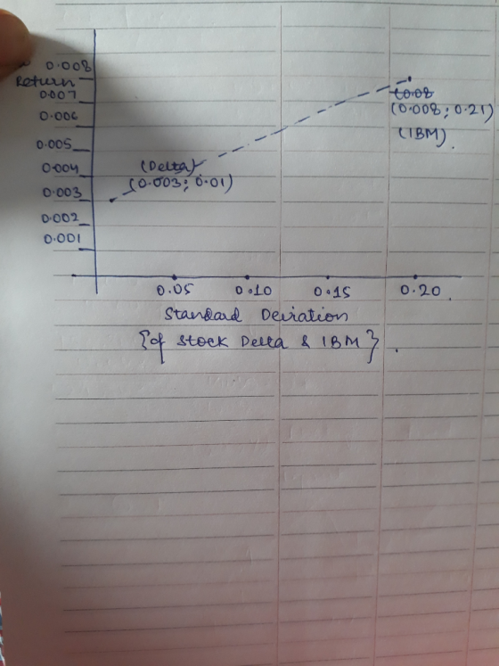
On the basis of above values, diagram of Mean and Standard deviation is as follows:

Now, lets do calculation of sharpe ratio.

For sharpe ratio it is informed that weights can be between -1 to 2. So all the possible portfolio mixes are here under:

	Delta	IBM
Mean	0.0033	0.0076
Standard Deviation (SD)	0.0089	0.2082
Case 1: Portfolio 1	Sell one stock of Delta and Buy Two stock of IBM
Weights	-1	2
Therefore,
	Delta	IBM	Total
Weighted Mean	-0.003283333	0.0152	0.011916667
Weighted SD	-0.008872274	0.416415051	0.407542777
Sharp Ratio	Weighted Mean- Risk Free Interest Rate
	Weighted SD
=	0.01191-0.0015
	0.4075
=	0.0104
	0.4075
=	0.0255		2nd Rank
Case 2: Portfolio 2	Buy One stock of IBM only
Weights	0	1
Therefore,
	Delta	IBM	Total
Weighted Mean	0	0.0076	0.0076
Weighted SD	0	0.2082	0.2082
Sharp Ratio	W(M)- Rf
	W( SD)
=	0.0076-0.0015
	0.2082
=	0.0061
	0.2082
=	0.0292		1st Rank
Case 3: Portfolio 3	Buy One stock of Delta only
Weights	1	0
Therefore,
	Delta	IBM	Total
Weighted Mean (W(M))	0.00328	0	0.00328
Weighted SD(W(SD))	0.0088	0	0.0088
Sharp Ratio	W (Mean)- Risk Free Interest Rate(Rf)
	W (SD)
=	0.00328-0.0015
	0.0088
=	0.00178
	0.0088
=	0.2009		3rd Rank
Case 4: Portfolio 4	Buy Two stock of Delta and Sell one stock of IBM
Weights	2	-1
Therefore,
	Delta	IBM	Total
Weighted Mean	0.00656	-0.0076	-0.00103
Weighted SD	0.0177	-0.2082	-0.1904
Sharp Ratio	W (M)- Rf
	W(SD)
=	-0.0025
	-0.1904
=	-0.0025
	-0.1904
=	0.01330		4th Rank

Conclusion: on the basis of above calculation we can conclude that if purchase of only one stock is possible then investor should go for Portfolio 2 i.e. invest all his funds in IBM stock only as it will provide highest Sharpe Ratio.

Otherwise, if it is mandatory to invest in both funds then investor should go for Portfolio 1 i.e. sell 1 stock of Delta and buy two stock of IBM.