A study in transportation safety collected data on 42 North American cities. From each city, two...
A study in transportation safety collected data on 42 North American cities. From each city, two of the variables recorded were explanatory variable x=percentage of licensed drivers who are under 21 years of age, and the response variable y=the number of fatal accidents per year per 1000 licenses. Of interest is the relationship between these two variables.
The data were analyzed in StatGraphics. Examine carefully the output below:
Regression Analysis - Linear model: Y = a + b*X
Parameter
Std. Estimate
Error
T Statistic
p-value
Intercept
-1.59741
0.371671
-4.29792
0.0001
Slope
0.287053
0.0293898
9.76711
0.0000
Correlation Coefficient = 0.839387
R-squared = 70.4571 percent
Standard error of estimate = 0.58935
Question 1 (3 points)
What is the correlation coefficient in this question, and what does
it indicate about the relationship between the number of fatal
accidents and the percentage of licensed drivers?
Homework Answers
From the given output,
Correlation coefficient = 0.839387
This correlation coefficient is very close to 1 which indicates that there is a strong positive association between number of fatal accidents and percentage of licensed drivers.
Add Answer to:
A study in transportation safety collected data on 42 North
American cities. From each city, two...
26) A study in transportation safety collected data on 42 North American cities. From each city,...
 26) A study in transportation safety collected data on 42 North American cities. From each city, two of the variables recorded were X = percentage of licensed drivers who are under 21 years of age, and Y = the number of fatal accidents per year per 1000 licenses. Below is the output from the data: Parameter Intercept Std. Estimate -1.59741 Error 0.371671 T Statistic -4.29792 p-value 0.0001 0.0293898 9.76711 0.0000 Slope 0.287053 Correlation coefficient = 0.839387 R-squared = 70.4571 percent...
City code %drivers21 fatal accidents/1000 1 12 1.309 2 5 0 3 12 2.539 4 9 2...
 city code
%drivers21
fatal accidents/1000
1
12
1.309
2
5
0
3
12
2.539
4
9
2.003
5
11
2.034
6
14
4.08
7
13
2.639
8
9
0.124
9
6
0
10
10
1.145
11
13
2.719
12
18
3.128
13
10
1.676
14
17
3.769
15
14
2.639
16
13
1.449
17
12
3.121
18
10
2.616
19
9
0.788
20
14
2.631
21
10
1.887
22
12
1
23
9
0.652
24
12
1.209
25
15
0.775...
city code
%drivers21
fatal accidents/1000
1
12
1.309
2
5
0
3
12
2.539
4
9
2.003
5
11
2.034
6
14
4.08
7
13
2.639
8
9
0.124
9
6
0
10
10
1.145
11
13
2.719
12
18
3.128
13
10
1.676
14
17
3.769
15
14
2.639
16
13
1.449
17
12
3.121
18
10
2.616
19
9
0.788
20
14
2.631
21
10
1.887
22
12
1
23
9
0.652
24
12
1.209
25
15
0.775...
34. Male versus Female Drivers The following data represent the number of licensed drivers in var...
 34. Male versus Female Drivers The following data represent the number of licensed drivers in various age groups and the number of fatal accidents within the age group by gender. Age Number of Number Number of Number Male Licensed of Fatal Female Licensed of Fatal Drivers (000s) Crashes Drivers (000s) Crashes 12 6.139 6,816 17664 20,063 19,984 4.441 8,400 5,375 227 5,180 5,016 8,595 7990 7,118 4,527 2,274 2.022 12 6,424 6,941 18,068 20,406 19,898 14,340 8,194 4,803 2,113 1.531...
Data were gathered from a simple random sample of cities. The variables are Violent Crime (crimes...
Data were gathered from a simple random sample of cities. The variables are Violent Crime (crimes per 100,000 population), Police Officer Wage (mean $/hr), and Graduation Rate (%). Use the accompanying regression table to answer the following questions consider the coefficient of Graduation Rate. Complete parts a through e Dependent variable is: Violent Crime R squared=36.1 R squared (adjusted)equals=38.2% s=129.6 with 37 degrees of freedom Variable Coeff SE (Coeff) t-ratio P-value Intercept 1391.86 187 .88 7.41 < 0.0001 Police Officer...
Solve the problem. What is the relationship between diamond price and carat size? 307 diamonds were...
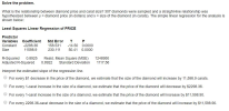 Solve the problem. What is the relationship between diamond price and carat size? 307 diamonds were sampled and a straight-line relationship was hypothesized between y = diamond price in dollars) and x = size of the diamond (in carats). The simple linear regression for the analysis is shown below: Least Squares Linear Regression of PRICE Predictor Variables Constant Size Coefficient -2298.36 11598.9 Std Error T P 158.531 -14.50 0.0000 230.111 50.41 0.0000 R-Squared 0.8925 Adjusted R-Squared Resid. Mean Square (MSE)...
4. Linear Regression [TOTAL 5 MARKS] McDonald (1989) collected the amphipod crustacean Platorchestia platensis on a...
 4. Linear Regression [TOTAL 5 MARKS] McDonald (1989) collected the amphipod crustacean Platorchestia platensis on a beach near Stony Brook, Long Island. He removed and counted the number of eggs for 28 females, and then freeze-dried and weighed the mothers (in mg) summary (1m (eggs~mass, eggdata) ) Call 1m (formula data eggdata) eggs mass, Coefficients: Estimate Std. Error t value Pr (>I t|) 12.6890 4.2009 3.021 0.0056 (Intercept) 1.6017 0.6176 2.593 0.0154 mass Signif. codes: 0* 0.001 0.01 0.05 .0.1...
1. The R codes and outputs shown below were obtained from a study of the relationship...
 1. The R codes and outputs shown below were obtained from a study of the relationship between heart rate (Y) and the body weight in kg (X). Assume that the linear regres- sion model Y, = Be + Bixi + Ei,i = 1,...,n where €; are i.i.d. N(0,0%) is appropriare for this data. We also assume di's as known constants. > xydata <- read.table("heart.txt", header = TRUE) > fit <- Im(YX, xydata) > summary(fit) Call: 1m(formula = Y - X,...
(1 point) College Graduation Rates. Data from the College Results Online website compared the 2011 graduation...
 (1 point) College Graduation Rates. Data from the College Results Online website compared the 2011 graduation rate and school size for 92 similar sized public universities and colleges in the United States. Statistical software was used to create the linear regression model using size as the explanatory variable and graduation rate as the response variable. Summary output from the software and the scatter plot are shown below. Round all calculated results to four decimal places Coefficients Estimate Std. Errort value...
Create the printout necessary for conducting a SLR analysis of your project data. Use y=price as...
Create the printout necessary for conducting a SLR analysis of your project data. Use y=price as your dependent variable and x=mileage/size as your independent variable. Copy and paste the printout here: Least Squares Linear Regression of Asking Predictor Variables Coefficient Std Error T P Constant 22790.9 1314.55 17.34 0.0000 Mileage -0.09109 0.03153 -2.89 0.0051 R² 0.1026 Mean Square Error (MSE) 1.102E+07 Adjusted R² 0.0903 Standard Deviation 3319.84 AICc 1220.5 PRESS 8.47E+08...
1 point) College Graduation Rates. Data from the College Results Online website compared the 2011...
 Hi! Can someone help me to calculate the last question, the CI?
Thanks!
1 point) College Graduation Rates. Data from the College Results Online website compared the 2011 graduation rate and school sze for 92 similar-sized public universities and colleges in the United States. Statistical sottware was used to places. create the linear regression model using size as the explanatory variable and graduation rate as the response variable. Summary output from the software and the scatter plot are shown below....
Hi! Can someone help me to calculate the last question, the CI?
Thanks!
1 point) College Graduation Rates. Data from the College Results Online website compared the 2011 graduation rate and school sze for 92 similar-sized public universities and colleges in the United States. Statistical sottware was used to places. create the linear regression model using size as the explanatory variable and graduation rate as the response variable. Summary output from the software and the scatter plot are shown below....
 26) A study in transportation safety collected data on 42 North American cities. From each city, two of the variables recorded were X = percentage of licensed drivers who are under 21 years of age, and Y = the number of fatal accidents per year per 1000 licenses. Below is the output from the data: Parameter Intercept Std. Estimate -1.59741 Error 0.371671 T Statistic -4.29792 p-value 0.0001 0.0293898 9.76711 0.0000 Slope 0.287053 Correlation coefficient = 0.839387 R-squared = 70.4571 percent...
 city code
%drivers21
fatal accidents/1000
1
12
1.309
2
5
0
3
12
2.539
4
9
2.003
5
11
2.034
6
14
4.08
7
13
2.639
8
9
0.124
9
6
0
10
10
1.145
11
13
2.719
12
18
3.128
13
10
1.676
14
17
3.769
15
14
2.639
16
13
1.449
17
12
3.121
18
10
2.616
19
9
0.788
20
14
2.631
21
10
1.887
22
12
1
23
9
0.652
24
12
1.209
25
15
0.775...
city code
%drivers21
fatal accidents/1000
1
12
1.309
2
5
0
3
12
2.539
4
9
2.003
5
11
2.034
6
14
4.08
7
13
2.639
8
9
0.124
9
6
0
10
10
1.145
11
13
2.719
12
18
3.128
13
10
1.676
14
17
3.769
15
14
2.639
16
13
1.449
17
12
3.121
18
10
2.616
19
9
0.788
20
14
2.631
21
10
1.887
22
12
1
23
9
0.652
24
12
1.209
25
15
0.775...
 34. Male versus Female Drivers The following data represent the number of licensed drivers in various age groups and the number of fatal accidents within the age group by gender. Age Number of Number Number of Number Male Licensed of Fatal Female Licensed of Fatal Drivers (000s) Crashes Drivers (000s) Crashes 12 6.139 6,816 17664 20,063 19,984 4.441 8,400 5,375 227 5,180 5,016 8,595 7990 7,118 4,527 2,274 2.022 12 6,424 6,941 18,068 20,406 19,898 14,340 8,194 4,803 2,113 1.531...
 Solve the problem. What is the relationship between diamond price and carat size? 307 diamonds were sampled and a straight-line relationship was hypothesized between y = diamond price in dollars) and x = size of the diamond (in carats). The simple linear regression for the analysis is shown below: Least Squares Linear Regression of PRICE Predictor Variables Constant Size Coefficient -2298.36 11598.9 Std Error T P 158.531 -14.50 0.0000 230.111 50.41 0.0000 R-Squared 0.8925 Adjusted R-Squared Resid. Mean Square (MSE)...
 4. Linear Regression [TOTAL 5 MARKS] McDonald (1989) collected the amphipod crustacean Platorchestia platensis on a beach near Stony Brook, Long Island. He removed and counted the number of eggs for 28 females, and then freeze-dried and weighed the mothers (in mg) summary (1m (eggs~mass, eggdata) ) Call 1m (formula data eggdata) eggs mass, Coefficients: Estimate Std. Error t value Pr (>I t|) 12.6890 4.2009 3.021 0.0056 (Intercept) 1.6017 0.6176 2.593 0.0154 mass Signif. codes: 0* 0.001 0.01 0.05 .0.1...
 1. The R codes and outputs shown below were obtained from a study of the relationship between heart rate (Y) and the body weight in kg (X). Assume that the linear regres- sion model Y, = Be + Bixi + Ei,i = 1,...,n where €; are i.i.d. N(0,0%) is appropriare for this data. We also assume di's as known constants. > xydata <- read.table("heart.txt", header = TRUE) > fit <- Im(YX, xydata) > summary(fit) Call: 1m(formula = Y - X,...
 (1 point) College Graduation Rates. Data from the College Results Online website compared the 2011 graduation rate and school size for 92 similar sized public universities and colleges in the United States. Statistical software was used to create the linear regression model using size as the explanatory variable and graduation rate as the response variable. Summary output from the software and the scatter plot are shown below. Round all calculated results to four decimal places Coefficients Estimate Std. Errort value...
 Hi! Can someone help me to calculate the last question, the CI?
Thanks!
1 point) College Graduation Rates. Data from the College Results Online website compared the 2011 graduation rate and school sze for 92 similar-sized public universities and colleges in the United States. Statistical sottware was used to places. create the linear regression model using size as the explanatory variable and graduation rate as the response variable. Summary output from the software and the scatter plot are shown below....
Hi! Can someone help me to calculate the last question, the CI?
Thanks!
1 point) College Graduation Rates. Data from the College Results Online website compared the 2011 graduation rate and school sze for 92 similar-sized public universities and colleges in the United States. Statistical sottware was used to places. create the linear regression model using size as the explanatory variable and graduation rate as the response variable. Summary output from the software and the scatter plot are shown below....
Most questions answered within 3 hours.
-
Where is the error in this code sequence?
String s1 = "Hello";
String s2 = "ello";...
asked 11 months ago -
Financial data for Joel de Paris, Inc., for last year
follow:
Joel de Paris, Inc.
Balance...
asked 11 months ago -
Consider this reaction:
Al2(SO4)3 (aq)+ BaCl3
(aq) Al2Cl6 (aq)- +
3BaSO4(s) . What is the...
asked 11 months ago -
Suppose that Savneet is considering increasing her
recent random sample from 20 car rentals to 40...
asked 11 months ago -
Trucks arrive at an unloading terminal at an average rate of 120
per hour.
Trucks arrive...
asked 11 months ago -
Why are methanol and ethanol completely soluble in water while
octanol is not very little soluble....
asked 11 months ago -
A facilities manager at a university reads in a research report
that the mean amount of...
asked 11 months ago -
When the CuSO4 is rehydrated by adding water to the anhydrous
compound, is this an endothermic...
asked 11 months ago -
A ray of sunlight is passing from diamond into crown glass; the
angle of incidence is...
asked 11 months ago -
A block of mass 0.249 kg is placed on top of a light, vertical
spring of...
asked 11 months ago -
how do the kidneys compensate in the presences of acidosis
a) trigger hyperventilate
b) reserve acid...
asked 11 months ago -
Question 501 pts
The rental rate of capital to the firm increases. Which of the
following...
asked 11 months ago