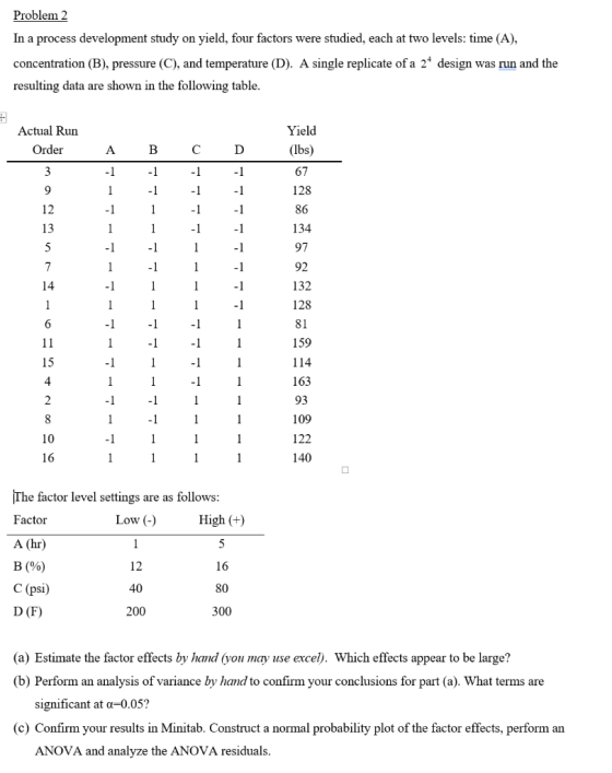
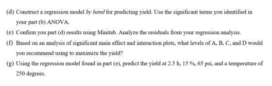
(d) Construct a regression model by hand for predicting yield. Use the significant terms you identified in your part (b) ANOVA (e) Confirm you part (d) results using Minitab. Analyze the residuals from your regression analysis (f) Based on an analysis of significant main effect and interaction plots, what levels of A, B, C, and D would you recommend using to maximize the yield? (g) Using the regression model found in part (e), predict the yield at 2.5 h, 15 % 65 psi and a temperature of 250 degrees
Homework Answers
Here we have given four factors each at two levels. The design is called 24 design.
The four factors are :
A : Time
B : Concentration
C : Pressure
D : Temperature.
First we have to construct 24 factorial design.
This we can done in MINITAB.
steps :
STAT --> DOE --> Factorial --> Create factorial design --> Type of design : 2-level factorial (default generators) --> Number of factors : 4 --> Designs --> Click on full factorial --> Number of center points per block : 0 --> Number of replicates for corner points : 1 --> Number of blocks : 1 --> ok --> Options : Store design in worksheet --> ok --> Results --> Printed results : Select last option --> ok --> ok
————— 7/6/2017 9:40:02 AM ————————————————————
Results for: Worksheet 4
Full Factorial Design
Factors: 4 Base Design: 4, 16
Runs: 16 Replicates: 1
Blocks: 1 Center pts (total): 0
All terms are free from aliasing.
Design Table
Run A B C D
1 - - - -
2 + - - -
3 - + - -
4 + + - -
5 - - + -
6 + - + -
7 - + + -
8 + + + -
9 - - - +
10 + - - +
11 - + - +
12 + + - +
13 - - + +
14 + - + +
15 - + + +
16 + + + +
Now we have to analyze this design.
steps :
ENTER data into MINITAB sheet --> Stat --> DOE --> Factorial --> ANalyze factorial design --> Responses : Select data column --> Terms : select --> ok --> Results --> Display of results: select 4th option --> Display of least squares means --> Selected terms : Select four factors --> ok --> ok
————— 7/6/2017 9:40:02 AM ————————————————————
Factorial Fit: observation versus A, B, C, D
Estimated Effects and Coefficients for observation (coded units)
Term Effect Coef SE Coef T P
Constant 37.875 0.7500 50.50 0.013
A 10.000 5.000 0.7500 6.67 0.095
B 0.750 0.375 0.7500 0.50 0.705
C 4.250 2.125 0.7500 2.83 0.216
D 6.750 3.375 0.7500 4.50 0.139
A*B -2.500 -1.250 0.7500 -1.67 0.344
A*C -9.000 -4.500 0.7500 -6.00 0.105
A*D 9.000 4.500 0.7500 6.00 0.105
B*C 0.250 0.125 0.7500 0.17 0.895
B*D -0.250 -0.125 0.7500 -0.17 0.895
C*D 0.250 0.125 0.7500 0.17 0.895
A*B*C 2.500 1.250 0.7500 1.67 0.344
A*B*D 1.500 0.750 0.7500 1.00 0.500
A*C*D -1.000 -0.500 0.7500 -0.67 0.626
B*C*D -1.750 -0.875 0.7500 -1.17 0.451
S = 3 R-Sq = 99.35% R-Sq(adj) = 90.29%
Analysis of Variance for observation (coded units)
Source DF Seq SS Adj SS Adj MS F P
Main Effects 4 656.75 656.750 164.187 18.24 0.174
2-Way Interactions 6 673.75 673.750 112.292 12.48 0.213
3-Way Interactions 4 50.25 50.250 12.562 1.40 0.555
Residual Error 1 9.00 9.000 9.000
Total 15 1389.75
Obs StdOrder observation Fit SE Fit Residual St Resid
1 1 26.0000 25.2500 2.9047 0.7500 1.00
2 2 40.0000 40.7500 2.9047 -0.7500 -1.00
3 3 30.0000 30.7500 2.9047 -0.7500 -1.00
4 4 34.0000 33.2500 2.9047 0.7500 1.00
5 5 37.0000 37.7500 2.9047 -0.7500 -1.00
6 6 33.0000 32.2500 2.9047 0.7500 1.00
7 7 43.0000 42.2500 2.9047 0.7500 1.00
8 8 33.0000 33.7500 2.9047 -0.7500 -1.00
9 9 21.0000 21.7500 2.9047 -0.7500 -1.00
10 10 55.0000 54.2500 2.9047 0.7500 1.00
11 11 28.0000 27.2500 2.9047 0.7500 1.00
12 12 52.0000 52.7500 2.9047 -0.7500 -1.00
13 13 41.0000 40.2500 2.9047 0.7500 1.00
14 14 47.0000 47.7500 2.9047 -0.7500 -1.00
15 15 37.0000 37.7500 2.9047 -0.7500 -1.00
16 16 49.0000 48.2500 2.9047 0.7500 1.00
Least Squares Means for observation
Mean SE Mean
A
-1 32.88 1.061
1 42.88 1.061
B
-1 37.50 1.061
1 38.25 1.061
C
-1 35.75 1.061
1 40.00 1.061
D
-1 34.50 1.061
1 41.25 1.061
A*C
-1 -1 26.25 1.500
1 -1 45.25 1.500
-1 1 39.50 1.500
1 1 40.50 1.500
A*D
-1 -1 34.00 1.500
1 -1 35.00 1.500
-1 1 31.75 1.500
1 1 50.75 1.500
B*C
-1 -1 35.50 1.500
1 -1 36.00 1.500
-1 1 39.50 1.500
1 1 40.50 1.500
B*D
-1 -1 34.00 1.500
1 -1 35.00 1.500
-1 1 41.00 1.500
1 1 41.50 1.500
C*D
-1 -1 32.50 1.500
1 -1 36.50 1.500
-1 1 39.00 1.500
1 1 43.50 1.500
A*B*C
-1 -1 -1 23.50 2.121
1 -1 -1 47.50 2.121
-1 1 -1 29.00 2.121
1 1 -1 43.00 2.121
-1 -1 1 39.00 2.121
1 -1 1 40.00 2.121
-1 1 1 40.00 2.121
1 1 1 41.00 2.121
A*B*D
-1 -1 -1 31.50 2.121
1 -1 -1 36.50 2.121
-1 1 -1 36.50 2.121
1 1 -1 33.50 2.121
-1 -1 1 31.00 2.121
1 -1 1 51.00 2.121
-1 1 1 32.50 2.121
1 1 1 50.50 2.121
A*C*D
-1 -1 -1 28.00 2.121
1 -1 -1 37.00 2.121
-1 1 -1 40.00 2.121
1 1 -1 33.00 2.121
-1 -1 1 24.50 2.121
1 -1 1 53.50 2.121
-1 1 1 39.00 2.121
1 1 1 48.00 2.121
B*C*D
-1 -1 -1 33.00 2.121
1 -1 -1 32.00 2.121
-1 1 -1 35.00 2.121
1 1 -1 38.00 2.121
-1 -1 1 38.00 2.121
1 -1 1 40.00 2.121
-1 1 1 44.00 2.121
1 1 1 43.00 2.121
Alias Structure
I
A
B
C
D
A*B
A*C
A*D
B*C
B*D
C*D
A*B*C
A*B*D
A*C*D
B*C*D
Overall significance :
Here test statistic follows F-distribution.
Here overall significance for the term main effects, 2-way interaction and 3-way interaction.
We see that all the three factors, 2-way interactions and 3-way interactions are insignificant.
Also we can see that all the terms are insignificant at 5% level of significance.
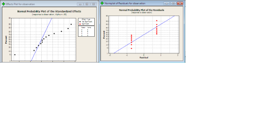
Here we can see from the normal probability plot the data follows normal distribution.
Add Answer to:
Problem 2 In a process development study on yield, four factors were studied, each at two levels:...
4. In a process development study on yield, four factors were studied, each at two levels: time (A), concentration (B),...
 4. In a process development study on yield, four factors were studied, each at two levels: time (A), concentration (B), pressure (C) and temperature (D). A single replicate of a 24 design was run, and the resulting are shown in the Table below a. Construct a normal probability plot of the effect estimates. Which factors appear to have large effects? b. Conduct an analysis of variance using the normal probability plot in part (a) for guidance in forming an error...
2. An experiment was run in a semiconductor fabrication plant in an effort to increase yield. Five factors, each at two levels, were studied. The factors (and levels) were A aperture setting (small,...
 2. An experiment was run in a semiconductor fabrication plant in an effort to increase yield. Five factors, each at two levels, were studied. The factors (and levels) were A aperture setting (small, large), B-exposure time (20% below nominal, 20% above nominal), C-development time (30s, 45s), D mask dimension (small, large), and E: etch time (145min, 15.5min). The unreplicated 25 design shown below was run. b 34 bd 32 be 35 bde 30 ab 55 abd 50 abe 52 abde...
1. An engineer is interested in the effects of cutting speed (A), tool geometry (B), and cutting angle (C) on the life (in hours) of a machine tool. Two levels of each factor are chosen, and three re...
 1. An engineer is interested in the effects of cutting speed (A), tool geometry (B), and cutting angle (C) on the life (in hours) of a machine tool. Two levels of each factor are chosen, and three replicates of a 23 factorial design are run. The results are as follows: Treatment Replicate A B CCombinationI 22 31 32 43 35 34 55 47 44 45 40 37 60 50 54 39 41 25 29 50 46 38 36 ac bc...
Problem 2 An experiment was conducted to determine the affects of temperature on the mean yield...
 Problem 2 An experiment was conducted to determine the affects of temperature on the mean yield of a chemical process. The data from the experiment (in the order collected) are shown in the following table Temperature (F) 300 550 500 300 250 375 300 250 500 550 375 500 450 375 550 450 250 450 Yield (mg) 25.0 36.3 25.9 21.8 29.4 19.6 33.2 25.1 26.2 38.3 12.7 39.1 21.8 17.5 35.1 26.3 30.5 19.3 a) Does temperature affect the...
6.5 An engineer is interested in the effects of cutting speed (A), tool geometry (B), and cutting...
 Solve parts b and d by using SPSS
6.5 An engineer is interested in the effects of cutting speed (A), tool geometry (B), and cutting angle (C) on the life (in hours) of a machine tool. Two levels of each factor are chosen, and three replicates of a 2 factorial design are run. The results are as follows: Replicate Treatment B C Combination 22 31 32 43 35 34 50 55 47 46 44 40 37 36 60 50 54...
Solve parts b and d by using SPSS
6.5 An engineer is interested in the effects of cutting speed (A), tool geometry (B), and cutting angle (C) on the life (in hours) of a machine tool. Two levels of each factor are chosen, and three replicates of a 2 factorial design are run. The results are as follows: Replicate Treatment B C Combination 22 31 32 43 35 34 50 55 47 46 44 40 37 36 60 50 54...
Solve parts b and d by using SPSS 6.5 An engineer is interested in the effects...
 Solve parts b and d by using SPSS
6.5 An engineer is interested in the effects of cutting speed (A), tool geometry (B), and cutting angle (C) on the life (in hours) of a machine tool. Two levels of each factor are chosen, and three replicates of a 2 factorial design are run. The results are as follows: Replicate Treatment B C Combination 22 31 32 43 35 34 50 55 47 46 44 40 37 36 60 50 54...
Solve parts b and d by using SPSS
6.5 An engineer is interested in the effects of cutting speed (A), tool geometry (B), and cutting angle (C) on the life (in hours) of a machine tool. Two levels of each factor are chosen, and three replicates of a 2 factorial design are run. The results are as follows: Replicate Treatment B C Combination 22 31 32 43 35 34 50 55 47 46 44 40 37 36 60 50 54...
4. An experiment was performed to improve the yield of a chemical process. Four factors, A, B, C and D were selected. Suppose that in the chemical process development experiment, it was only possible...
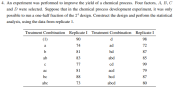 4. An experiment was performed to improve the yield of a chemical process. Four factors, A, B, C and D were selected. Suppose that in the chemical process development experiment, it was only possible to run a one-half fraction of the 24 design. Construct the design and perform the statistical analysis, using the data from replicate 1 Treatment Combination Replicate I 90 74 81 83 Treatment Combination Replicate I 98 72 87 85 ad bd cd 81 79 87 ac...
6.6.Reconsider the experiment described in Problem 6.1 Suppose that the experimenter only perform...
 6.6.Reconsider the experiment described in Problem 6.1 Suppose that the experimenter only performed the eight trials from replicate I. In addition, he ran four center points and obtained the following response values: 36, 40, 43, 45 (a) Estimate the factor effects. Which effects are large? (b) Perform an analysis of variance, including a check for pure quadratic curvature. What are your conclusions? (c) Write down an appropriate model for predicting tool life, based on the results of this experiment. Does...
An article in Environment International describes an experiment in which the amount of radon released in...
 An article in Environment International describes an experiment in which the amount of radon released in showers was investigated. Radon-enriched water was used in the experiment, and six different orifice diameters were tested in shower heads. The data from the experiment (in the order collected) are shown in the following table. Orifice Diameter (mm) | 140 51 37 51 102 51 199 102 102 51 140 37 37 71 140 140 71 102 37 199 51 71 199 140 37...
Question #2 (30 points) The yield of a chemical process is being studied. The two most important ...
 Question #2 (30 points) The yield of a chemical process is being studied. The two most important variables a thought to be the pressure and the temperature. Three levels of each factor are selected, and a factorial experiment with two replicates is performed. The yield data are as follows: Pressure (psig) Temperature (C) 150 200 90.4 90.2 90.1 90.3 90.5 90.7 215 90.7 90.6 90.5 90.6 90.8 90.9 230 90.2 90.4 89.9 90.1 90.4 90.1 160 170 a. Write the...
 4. In a process development study on yield, four factors were studied, each at two levels: time (A), concentration (B), pressure (C) and temperature (D). A single replicate of a 24 design was run, and the resulting are shown in the Table below a. Construct a normal probability plot of the effect estimates. Which factors appear to have large effects? b. Conduct an analysis of variance using the normal probability plot in part (a) for guidance in forming an error...
 2. An experiment was run in a semiconductor fabrication plant in an effort to increase yield. Five factors, each at two levels, were studied. The factors (and levels) were A aperture setting (small, large), B-exposure time (20% below nominal, 20% above nominal), C-development time (30s, 45s), D mask dimension (small, large), and E: etch time (145min, 15.5min). The unreplicated 25 design shown below was run. b 34 bd 32 be 35 bde 30 ab 55 abd 50 abe 52 abde...
 1. An engineer is interested in the effects of cutting speed (A), tool geometry (B), and cutting angle (C) on the life (in hours) of a machine tool. Two levels of each factor are chosen, and three replicates of a 23 factorial design are run. The results are as follows: Treatment Replicate A B CCombinationI 22 31 32 43 35 34 55 47 44 45 40 37 60 50 54 39 41 25 29 50 46 38 36 ac bc...
 Problem 2 An experiment was conducted to determine the affects of temperature on the mean yield of a chemical process. The data from the experiment (in the order collected) are shown in the following table Temperature (F) 300 550 500 300 250 375 300 250 500 550 375 500 450 375 550 450 250 450 Yield (mg) 25.0 36.3 25.9 21.8 29.4 19.6 33.2 25.1 26.2 38.3 12.7 39.1 21.8 17.5 35.1 26.3 30.5 19.3 a) Does temperature affect the...
 Solve parts b and d by using SPSS
6.5 An engineer is interested in the effects of cutting speed (A), tool geometry (B), and cutting angle (C) on the life (in hours) of a machine tool. Two levels of each factor are chosen, and three replicates of a 2 factorial design are run. The results are as follows: Replicate Treatment B C Combination 22 31 32 43 35 34 50 55 47 46 44 40 37 36 60 50 54...
Solve parts b and d by using SPSS
6.5 An engineer is interested in the effects of cutting speed (A), tool geometry (B), and cutting angle (C) on the life (in hours) of a machine tool. Two levels of each factor are chosen, and three replicates of a 2 factorial design are run. The results are as follows: Replicate Treatment B C Combination 22 31 32 43 35 34 50 55 47 46 44 40 37 36 60 50 54...
 Solve parts b and d by using SPSS
6.5 An engineer is interested in the effects of cutting speed (A), tool geometry (B), and cutting angle (C) on the life (in hours) of a machine tool. Two levels of each factor are chosen, and three replicates of a 2 factorial design are run. The results are as follows: Replicate Treatment B C Combination 22 31 32 43 35 34 50 55 47 46 44 40 37 36 60 50 54...
Solve parts b and d by using SPSS
6.5 An engineer is interested in the effects of cutting speed (A), tool geometry (B), and cutting angle (C) on the life (in hours) of a machine tool. Two levels of each factor are chosen, and three replicates of a 2 factorial design are run. The results are as follows: Replicate Treatment B C Combination 22 31 32 43 35 34 50 55 47 46 44 40 37 36 60 50 54...
 4. An experiment was performed to improve the yield of a chemical process. Four factors, A, B, C and D were selected. Suppose that in the chemical process development experiment, it was only possible to run a one-half fraction of the 24 design. Construct the design and perform the statistical analysis, using the data from replicate 1 Treatment Combination Replicate I 90 74 81 83 Treatment Combination Replicate I 98 72 87 85 ad bd cd 81 79 87 ac...
 6.6.Reconsider the experiment described in Problem 6.1 Suppose that the experimenter only performed the eight trials from replicate I. In addition, he ran four center points and obtained the following response values: 36, 40, 43, 45 (a) Estimate the factor effects. Which effects are large? (b) Perform an analysis of variance, including a check for pure quadratic curvature. What are your conclusions? (c) Write down an appropriate model for predicting tool life, based on the results of this experiment. Does...
 An article in Environment International describes an experiment in which the amount of radon released in showers was investigated. Radon-enriched water was used in the experiment, and six different orifice diameters were tested in shower heads. The data from the experiment (in the order collected) are shown in the following table. Orifice Diameter (mm) | 140 51 37 51 102 51 199 102 102 51 140 37 37 71 140 140 71 102 37 199 51 71 199 140 37...
 Question #2 (30 points) The yield of a chemical process is being studied. The two most important variables a thought to be the pressure and the temperature. Three levels of each factor are selected, and a factorial experiment with two replicates is performed. The yield data are as follows: Pressure (psig) Temperature (C) 150 200 90.4 90.2 90.1 90.3 90.5 90.7 215 90.7 90.6 90.5 90.6 90.8 90.9 230 90.2 90.4 89.9 90.1 90.4 90.1 160 170 a. Write the...
Most questions answered within 3 hours.
-
Where is the error in this code sequence?
String s1 = "Hello";
String s2 = "ello";...
asked 11 months ago -
Financial data for Joel de Paris, Inc., for last year
follow:
Joel de Paris, Inc.
Balance...
asked 11 months ago -
Consider this reaction:
Al2(SO4)3 (aq)+ BaCl3
(aq) Al2Cl6 (aq)- +
3BaSO4(s) . What is the...
asked 11 months ago -
Suppose that Savneet is considering increasing her
recent random sample from 20 car rentals to 40...
asked 11 months ago -
Trucks arrive at an unloading terminal at an average rate of 120
per hour.
Trucks arrive...
asked 11 months ago -
Why are methanol and ethanol completely soluble in water while
octanol is not very little soluble....
asked 11 months ago -
A facilities manager at a university reads in a research report
that the mean amount of...
asked 11 months ago -
When the CuSO4 is rehydrated by adding water to the anhydrous
compound, is this an endothermic...
asked 11 months ago -
A ray of sunlight is passing from diamond into crown glass; the
angle of incidence is...
asked 11 months ago -
A block of mass 0.249 kg is placed on top of a light, vertical
spring of...
asked 11 months ago -
how do the kidneys compensate in the presences of acidosis
a) trigger hyperventilate
b) reserve acid...
asked 11 months ago -
Question 501 pts
The rental rate of capital to the firm increases. Which of the
following...
asked 11 months ago