Question

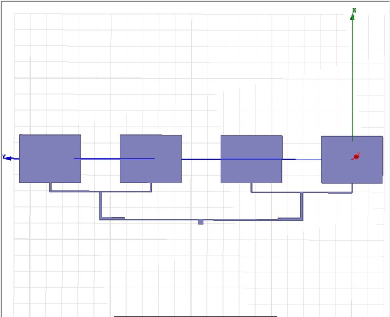
Design H -SHAPE microstrip array antenna in HFSS software and MATLAB CODE FOR IT.

I NEED ALL THE OUTPUT FOR THIS CODE

IF YOU KNOW THEN ONLY DO OR ELSE LEAVE FOR OTHER

ANTENNA ,ELECTRICAL ENGINEERING

Answer 1

dB (GainTotal) 2. 4101e+000 1.6807e+000 9. 5134e-001 2.2198e-001 -5.0739e-001 -1.2368e+000 1.9661e+000 -2. 6955e+000 3.4248e+000 -4. 1542e+000 -4, 8836e+000 5. 6129e+000 -6, 3423e+000 7.0717e+000 7. 8010e+000 8.5304e +000 9. 2597e+000 2

XY Plot.3 HFSSDesign1 ▲ Name m1 0.0000 2.4101 Curve Info dB(GainTotal) Setup1 LastAdaptive Freq 2.4GHz Phi Odeg dB(GainTotal) Setup1 LastAdaptive Freq-2.4GHz' Phi-90deg 0.00 2.50 5.00 7.50 10.00 -50.00 50.00 Theta [deg]

%*******************************************************************
% MICROSTRIP
%*******************************************************************
% THIS PROGRAM IS A MATLAB PROGRAM THAT DESIGNS AND THEN COMPUTES THE
% ANTENNA RADIATION CHARACTERISTICS OF:
%
%     I.   RECTANGULAR
%     II. CIRCULAR
%
% MICROSTRIP PATCH ANTENNAS BASED ON THE CAVITY MODEL AND DOMINANT
% MODE OPERATION FOR EACH. THAT IS:
%
%     A. TM(010) MODE FOR THE RECTANGULAR PATCH
%     B. TM(011) MODE FOR THE CIRCULAR PATCH
%
%     ** INPUT PARAMETERS
%     1. FREQ   = RESONANT FREQUENCY (in GHz)
%     2. EPSR   = DIELECTRIC CONSTANT OF THE SUBSTRATE
%     3. HEIGHT = HEIGHT OF THE SUBSTRATE (in cm)
%     4. Y0     = POSITION OF THE RECESSED FEED POINT (in cm)
%                  RELATIVE TO LEADING RADIATING EDGE OF RECTANGULAR
%                  PATCH. NOT NECESSARY FOR CIRCULAR PATCH.
%
%     ** OUTPUT PARAMETERS
%     A. RECTANGULAR PATCH:
%
%         1. PHYSICAL WIDTH OF THE PATCH W (in cm)
%         2. EFFECTIVE LENGTH OF PATCH Le (in cm)
%         3. PHYSICAL LENGTH OF PATCH L (in cm)
%         4. NORMALIZED E-PLANE AMPLITUDE PATTERN (in dB)
%         5. NORMALIZED H-PLANE AMPLITUDE PATTERN (in dB)
%         6. E-PLANE HALF-POWER BEAMWIDTH (in degrees)
%         7. H-PLANE HALF-POWER BEAMWIDTH (in degrees)
%         8. DIRECTIVITY (dimensionless and in dB)
%         9. RESONANT INPUT RESISTANCE (in ohms)
%             a. AT LEADING RADIATING EDGE (y = 0)
%             b. AT RECESSED FEED POINT FROM LEADING RADIATING EDGE
%                 (y = yo)
%
%     B. CIRCULAR PATCH:
%
%         1. PHYSICAL RADIUS OF THE PATCH a (in cm)
%         2. EFFECTIVE RADIUS OF THE PATCH ae (in cm)
%         3. NORMALIZED E-PLANE AMPLITUDE (in dB)
%         4. NORMALIZED H-PLANE AMPLITUDE (in dB)
%         5. E-PLANE HALF-POWER BEAMWIDTH (in degrees)
%         6. H-PLANE HALF-POWER BEAMWIDTH (in degrees)
%         7. DIRECTIVITY (dimensionless and in dB)
%
%*******************************************************************
%     Programmed by : Sung-Woo Lee , Arizona State University
%     Modified by   : Zhiyong Huang, Arizona State University
%     Nov. 23, 2004
%*******************************************************************

function []=MICROSTP;
clear all;
close all;
warning off;

option=[];
while isempty(option)|(option~=1&option~=2),
   option=input(['SELECT OUTPUT METHOD\n','   OPTION (1): SCREEN\n','   OPTION (2): OUTPUT FILE\n', ...
                 'SELECT OPTION: ']);
end;      

filename=[];
if option==2,
   while isempty(filename),
      filename=input('INPUT THE DESIRED OUTPUT FILENAME <in single quotes> = ','s');
   end;
end;

addpath(pwd);

if exist(filename,'file')&isa(filename,'char'),
   delete(filename);
end;
rmpath(pwd);

patchm=[];
while isempty(patchm)|((patchm~=1)&(patchm~=2)),
   patchm=input(['PATCH GEOMETRY OPTION\n','   OPTION (1) : RECTANGULAR PATCH\n', ...
                '   OPTION (2) : CIRCULAR PATCH\n','SELECT OPTION NUMBER: ']);
end;

if (patchm==1),           % Rectangular
   rect(option,filename);
else % Circular  
   circ(option,filename);
end;

warning on;

%%%%%%%%%%%%%%%%%%%
function rect=rect(option_a,filename);
%%%%%%%%%%%%%%%%%%%

% Input Parameters (freq, epsr, height, Yo)
freq=[];
while isempty(freq),
   freq=input('INPUT THE RESONANT FREQUENCY (in GHz) = ');
end;

er=[];
while isempty(er),
   er=input('INPUT THE DIELECTRIC CONSTANT OF THE SUBSTRATE = ');
end;

h=[];
while isempty(h),
   h=input('INPUT THE HEIGHT OF THE SUBSTRATE (in cm) = ');
end;

option1=[];
while isempty(option1)|(option1~=1&option1~=2),
   option1=input(['OPTIONS \n','   OPTION (1): FIND INPUT IMPEDANCE Zin AT FEED-POINT Yo \n', ...
                 '   OPTION (2): DETERMINE Yo FOR A GIVEN DESIRED Zin \n', ...
                 'SELE1CT OPTION NUMBER: ']);
end;

if option1==1
    Yo=[];
    while isempty(Yo),
        Yo=input(['\nINPUT THE POSITION OF THE RECESSED FEED POINT ' ...
                  'RELATIVE TO THE LEADING RADIATING EDGE\n' 'OF THE RECTANGULAR PATCH (in cm) = ']);
      
    end
else
    Zin=[];
    while isempty(Zin),
        Zin=input(['INPUT THE DESIRED INPUT IMPEDANCE Zin (in ohms) = ']);
    end
end

% Compute W, ereff, Leff, L (in cm)
W=30.0/(2.0*freq)*sqrt(2.0/(er+1.0));
ereff=(er+1.0)/2.0+(er-1)/(2.0*sqrt(1.0+12.0*h/W));
dl=0.412*h*((ereff+0.3)*(W/h+0.264))/((ereff-0.258)*(W/h+0.8));
lambda_o=30.0/freq;
lambda=30.0/(freq*sqrt(ereff));
Leff=30.0/(2.0*freq*sqrt(ereff));
L=Leff-2.0*dl;
ko=2.0*pi/lambda_o;
Emax=sinc(h*ko/2.0/pi);

% Normalized radiated field
%         E-plane pattern : 0 < phi < 90    ;    270 < phi < 360
%         H-plane pattern : 0 < th < 180

phi=0:360; phir=phi.*pi./180; [Ethval,Eth]=E_th(phir,h,ko,Leff,Emax);

th=0:360; thr=th.*pi/180.0;    [Ephval,Eph1]=E_ph(thr,h,ko,W,Emax);
Eph(1:91)=Eph1(91:181); Eph(91:270)=Eph1(181); Eph(271:361)=Eph1(1:91);

% Output files
fid_e=fopen('Epl-Micr_m.dat','wt');
fid_h=fopen('Hpl-Micr_m.dat','wt');
fprintf(fid_e,'# E-PLANE RADIATION PATTERN\n');
fprintf(fid_e,'# -------------------------\n#\n');
fprintf(fid_h,'# H-PLANE RADIATION PATTERN\n');
fprintf(fid_h,'# NOTE: THIS PATTERN IS ROTATED CCW BY 90 DEGREES\n');
fprintf(fid_h,'# -------------------------\n#\n');

Epl=[phi;Eth];
fprintf(fid_e,' %7.4f\t%7.4f\n',Epl);
fclose(fid_e);
Hpl=[[0:90 270:360];[Eph(1:91) Eph(271:361)]];
fprintf(fid_h,' %7.4f\t%7.4f\n',Hpl);
fclose(fid_h);

% Plots of Radiation Patterns
% Figure 1
% ********
Etheta=[Eth(271:361),Eth(2:91)];
xs=[0 20 40 60 80 90 100 120 140 160 180];
xsl=[270 290 310 330 350 0 10 30 50 70 90];
hli1=plot(Etheta,'b-');
set(gca,'Xtick',xs);
set(gca,'Xticklabel',xsl);
set(gca,'position',[0.13 0.11 0.775 0.8]);
h1=gca; h2=copyobj(h1,gcf);
xlim([0 180]);ylim([-60 0]);
set(h1,'xcolor',[0 0 1]); set(hli1,'erasemode','xor'); hx=xlabel('\phi (degrees)','fontsize',12);

axes(h2); hli2=plot(Eph1,'r:'); axis([0 180 -60 0]);
set(h2,'xaxislocation','top','xcolor',[1 0 0]);
legend([hli1 hli2],{'E_{\phi} (E-plane)','E_{\phi} (H-plane)'},4);
xlabel('\theta (degrees)','fontsize',12);

set([hli1 hli2],'linewidth',2); set(hx,'erasemode','xor');
ylabel('Radiation patterns (in dB)','fontsize',12);
% title('E- and H-plane Patterns of Rectangular Microstrip Antenna','fontsize',[12]);

% Figure 2
% ********
figure(2);
hp1=semipolar_micror(phir,Eth,-60,0,4,'-','b'); hold on;
hp2=semipolar_micror(phi*pi/180,Eph,-60,0,4,':','r');
title('E- and H-plane Patterns of Rectangular Microstrip Antenna','fontsize',[12]);
hle=legend([hp1 hp2],{'E_{\phi} (E-plane)','E_{\phi} (H-plane)'},0);

% E-plane HPBW and H-plane HPBW
% ******************************
an=phi(Eth>-3);
an(an>90)=[];

EHPBW=2*abs(max(an));
HHPBW=2*abs(90-min(th(Eph1>-3)));

% Directivity
[D,DdB]=dir_rect(W,h,Leff,L,ko);

% Input Impedance at Y=0 and Y=Yo
[G1,G12]=sintegr(W,L,ko);
Rin0P=(2.*(G1+G12))^-1;
Rin0M=(2.*(G1-G12))^-1;
if option1==1
    RinYoP=Rin0P*cos(pi*Yo/L)^2;
    RinYoM=Rin0M*cos(pi*Yo/L)^2;
else
    YP=acos(sqrt(Zin/Rin0P))*L/pi;
    YM=acos(sqrt(Zin/Rin0M))*L/pi;
end

% Display (rectangular)
clc;
if(option_a==2)
   diary(filename);
end
disp(strvcat('INPUT PARAMETERS','================'));
disp(sprintf('\nRESONANT FREQUENCY (in GHz) = %4.4f',freq));
disp(sprintf('DIELECTRIC CONSTANT OF THE SUBSTRATE = %4.4f',er));
disp(sprintf('HEIGHT OF THE SUBSTRATE (in cm) = %4.4f',h));
if option1==1
    disp(sprintf('POSITION OF THE RECESSED FEED POINT (in cm) = %4.4f\n',Yo));
else
    fprintf('DESIRED RESONANT INPUT INPEDANCE (in ohms) = %4.4f\n', Zin);
end
disp(strvcat('OUTPUT PARAMETERS','================='));
disp(sprintf('\nPHYSICAL WIDTH OF PATCH (in cm) = %4.4f',W));
disp(sprintf('EFFECTIVE LENGH OF PATCH (in cm) = %4.4f',Leff));
disp(sprintf('PHYSICAL LENGH OF PATCH (in cm) = %4.4f',L));
disp(sprintf('E-PLANE HPBW (in degrees) = %4.4f',EHPBW));
disp(sprintf('H-PLANE HPBW (in degrees) = %4.4f',HHPBW));
disp(sprintf('DIRECTIVITY OF RECTANGULAR PATCH (dimensionless) = %4.4f',D));
disp(sprintf('DIRECTIVITY OF RECTANGULAR PATCH (in dB) = %4.4f\n',DdB));

disp(sprintf('G1 (Using (14-12)) = %4.8f', G1));
disp(sprintf('G12 (Using (14-18a)) = %4.8f\n', G12));

disp(sprintf('RESONANT INPUT RESISTANCE AT LEADING RADIATING EDGE (y=0) Rin0P (Using + sign in (14-17)) = %4.4f ohms',Rin0P));
disp(sprintf('RESONANT INPUT RESISTANCE AT LEADING RADIATING EDGE (y=0) Rin0M (Using - sign in (14-17)) = %4.4f ohms\n',Rin0M));

if option1==1
    fprintf('RESONANT INPUT RESISTANCE AT RECESSED FEED POINT (y=%4.4f cm) RinYoP (Using + sign in (14-17)) = %4.4f ohms\n',Yo, RinYoP);
    fprintf('RESONANT INPUT RESISTANCE AT RECESSED FEED POINT (y=%4.4f cm) RinYoM (Using - sign in (14-17)) = %4.4f ohms\n\n',Yo, RinYoM);
else
    fprintf('FOR DESIRED IMPENDANCE %4.4f ohms, THE FEED POINT POSITION YoP (Using + sign in (14-17)) = %4.4f cm\n',Zin, YP);
    fprintf('FOR DESIRED IMPENDANCE %4.4f ohms, THE FEED POINT POSITION YoM (Using - sign in (14-17)) = %4.4f cm\n\n',Zin, YM);
end

disp(strvcat('*** NOTE:',...
   '    THE E-PLANE AMPLITUDE PATTERN IS STORED IN Epl-Micr_m.dat',...
   '    THE H-PLANE AMPLITUDE PATTERN IS STORED IN Hpl-Micr_m.dat',...
   '    ========================================================='));
diary off;

% Subfunctions
% ************
function [Ethval,Eth]=E_th(phir,h,ko,Leff,Emax)
ARG=cos(phir).*h.*ko./2;
Ethval=(sinc(ARG./pi).*cos(sin(phir).*ko*Leff./2))./Emax;
Eth=20*log10(abs(Ethval));
Eth(phir>pi/2&phir<3*pi/2)=-60;
Eth(Eth<=-60)=-60;

function [Ephval,Eph1]=E_ph(thr,h,ko,W,Emax)
ARG1=sin(thr).*h.*ko./2;
ARG2=cos(thr).*W.*ko./2;
Ephval=sin(thr).*sinc(ARG1./pi).*sinc(ARG2./pi)./Emax;
Eph1=20.0*log10(abs(Ephval));
Eph1(Eph1<=-60)=-60;

function [D,DdB]=dir_rect(W,h,Leff,L,ko)
th=0:180; phi=[0:90 270:360];
[t,p]=meshgrid(th.*pi/180,phi.*pi/180);
X=ko*h/2*sin(t).*cos(p);
Z=ko*W/2*cos(t);
Et=sin(t).*sinc(X/pi).*sinc(Z/pi).*cos(ko*Leff/2*sin(t).*sin(p));
U=Et.^2;
dt=(th(2)-th(1))*pi/180;
dp=(phi(2)-phi(1))*pi/180;
Prad=sum(sum(U.*sin(t)))*dt*dp;
D=4.*pi.*max(max(U))./Prad;
DdB=10.*log10(D);

function [G1,G12]=sintegr(W,L,ko)
th=0:1:180; t=th.*pi/180;
ARG=cos(t).*(ko*W/2);
res1=sum(sinc(ARG./pi).^2.*sin(t).^2.*sin(t).*((pi/180)*(ko*W/2)^2));
res12=sum(sinc(ARG./pi).^2.*sin(t).^2.*besselj(0,sin(t).*(ko*L)).*sin(t).*((pi/180)*(ko*W/2)^2));
G1=res1./(120*pi^2); G12=res12./(120*pi^2);

%%%%%%%%%%%%%%%%%%%
function circ=circ(option_a,filename);
%%%%%%%%%%%%%%%%%%%

% Input Parameters (freq, epsr, height)
freq=[];
while isempty(freq),
   freq=input('INPUT THE RESONANT FREQUENCY (in GHz) = ');
end;

er=[];
while isempty(er),
   er=input('INPUT THE DIELECTRIC CONSTANT OF THE SUBSTRATE = ');
end;

h=[];
while isempty(h),
   h=input('INPUT THE HEIGHT OF THE SUBSTRATE (in cm) = ');
end;

con=input('PLEASE INPUT THE CONDUCTIVITY (DEFAULT VALUE IS 10^7):');
if isempty(con)
    con=10^7;
end

lt=input('PLEASE INPUT THE LOST TANGENT (DEFAULT VALUE OF DOMNINANT MODE TM110 IS 0.0018):');
if isempty(lt)
    lt=0.0018;
end

%input of the rho0 or zin
option1=[];
while isempty(option1)|(option1~=1&option1~=2),
   option1=input(['OPTIONS \n','   OPTION (1): FIND INPUT IMPEDANCE Zin AT FEED-POINT RHOo \n', ...
                 '   OPTION (2): DETERMINE RHOo FOR A GIVEN DESIRED Zin \n', ...
                 'SELE1CT OPTION NUMBER: ']);
end;

if option1==1
    RHOo=[];
    while isempty(RHOo),
        RHOo=input(['\nINPUT THE POSITION OF THE RECESSED FEED POINT ' ...
                  'RELATIVE TO THE CENTER OF THE CIRCULAR PATCH (in cm) = ']);
      
    end
else
    Zin=[];
    while isempty(Zin),
        Zin=input(['INPUT THE DESIRED INPUT IMPEDANCE Zin (in ohms) = ']);
    end
end

% Compute the Physical Radius a (in cm) and Effective Radius ae (in cm)
lambda_o=30.0/freq;
ko=2.0*pi/lambda_o;
F=8.791/(freq*sqrt(er));
a=F/sqrt(1+2*h/(pi*er*F)*(log(pi*F/(2*h))+1.7726));
ae=a*sqrt(1+2*h/(pi*er*a)*(log(pi*a/(2*h))+1.7726));

% Normalized radiated field
%         E-plane and H-plane patterns : 0 < th < 90
th=0:90; thr=th.*pi./180;
x=sin(thr).*ko.*ae;
J0=besselj(0,x);
J2=besselj(2,x);
Eth1=J0-J2;
Eph1=(J0+J2).*cos(thr);

Eth2=20.*log10(Eth1./max(Eth1));
Eph2=20.*log10(Eph1./max(Eph1));
Eth2(Eth2<=-60)=-60;
Eph2(Eph2<=-60)=-60;

Eth(1:91)=Eth2(1:91); Eth(91:270)=Eth2(91); Eth(271:361)=Eth2(91:-1:1);
Eph(1:91)=Eph2(1:91); Eph(91:270)=Eph2(91); Eph(271:361)=Eph2(91:-1:1);

% Output files
fid_e=fopen('Epl-Micr_m.dat','wt');
fid_h=fopen('Hpl-Micr_m.dat','wt');
fprintf(fid_e,'# E-PLANE RADIATION PATTERN\n');
fprintf(fid_e,'# -------------------------\n#\n');
fprintf(fid_h,'# H-PLANE RADIATION PATTERN\n');
fprintf(fid_h,'# -------------------------\n#\n');

Epl=[[0:90 270:360];[Eth(1:91) Eth(271:361)]];
fprintf(fid_e,' %7.4f\t%7.4f\n',Epl);
fclose(fid_e);
Hpl=[[0:90 270:360];[Eph(1:91) Eph(271:361)]];
fprintf(fid_h,' %7.4f\t%7.4f\n',Hpl);
fclose(fid_h);

% Plots of Radiation Patterns
phi=0:360;

% Figure 1
% ********
hli1=plot(-90:90,[fliplr(Eth2) Eth2(2:end)],'b-'); set(gca,'position',[0.13 0.11 0.775 0.8]);
h1=gca; h2=copyobj(h1,gcf); axis([-90 90 -60 0]);
set(h1,'xcolor',[0 0 1]); set(hli1,'erasemode','xor'); hx=xlabel('\theta (degrees)','fontsize',12);

axes(h2); hli2=plot(-90:90,[fliplr(Eph2) Eph2(2:end)],'r:'); axis([-90 90 -60 0]);
set(h2,'xaxislocation','top','xcolor',[1 0 0]);
set([hli1 hli2],'linewidth',2);
legend([hli1 hli2],{'E_{\theta} (E-plane)','E_{\phi} (H-plane)'},4);
xlabel('\theta (degrees)','fontsize',12);

% Figure 2
% ********
figure(2);
thr=(-90:90)*pi/180;
hp1=semipolar_microc(thr,[fliplr(Eth2) Eth2(2:end)],-60,0,4,'-','b'); hold on;
hp2=semipolar_microc(thr,[fliplr(Eph2) Eph2(2:end)],-60,0,4,':','r');
hle=legend([hp1 hp2],{'E_{\theta} (E-plane)','E_{\phi} (H-plane)'},0);
title('E- and H-plane Patterns of Circular Microstrip Antenna','fontsize',[12]);

% E-plane and H-plane HPBW
an=th(Eth2>-3);
bn=th(Eph2>-3);

EHPBW=2*abs(max(an));
HHPBW=2*abs(max(bn));

%resonant input resistance
t=[0:0.001:pi/2];
x=ko*ae*sin(t);
j0=besselj(0,x);
j2=besselj(2,x);
j02p=j0-j2;
j02=j0+j2;
grad=(ko*ae)^2/480*sum((j02p.^2+(cos(t)).^2.*j02.^2).*sin(t).*0.001);

emo=1;
m=1;
mu0=4*pi*10^(-7);
k=ko*sqrt(er);

gc=emo*pi*(pi*mu0*freq*10^9)^(-3/2)*((k*ae)^2-m^2)/(4*(h/100)^2*sqrt(con));

gd=emo*lt*((k*ae)^2-m^2)/(4*mu0*h/100*freq*10^9);

gt=grad+gc+gd;
Rin0=1/gt;

if option1==1
    Rin=Rin0*besselj(1,k*RHOo)^2/besselj(1,k*ae)^2;
else
    temp1=Zin/Rin0*besselj(1,k*ae)^2;
    maxrho=ae;
    minrho=0;
    tempk=1;
    while tempk>0.00001
        nk=0;
        rhox=linspace(minrho,maxrho,100);
        temp=besselj(1,k.*rhox).^2;
        for kk=1:99
            if temp(kk)-temp1<=0
                if temp(kk+1)-temp1>0
                    nk=nk+1;
                    minrho=rhox(kk);
                    maxrho=rhox(kk+1);
                end
            else
                if temp(kk+1)-temp1<=0
                    nk=nk+1;
                    maxrho=rhox(kk);
                    minrho=rhox(kk+1);
                end
            end
        end
        if nk>1
            display('*****Warning, there are more than one solutions for RHOo and this program only provides you one exact solution!*****/n');
        end
        [tempk,kk]=min(abs(temp-temp1));
        RHOo=rhox(kk);
    end
end

% Directivity
[D,DdB]=dir_cir(a,ae,ko);

% Display (circular)
clc;
if (option_a==2),
   diary(filename);
end

disp(strvcat('INPUT PARAMETERS','================'));
disp(sprintf('\nRESONANT FREQUENCY (in GHz) = %4.4f',freq));
disp(sprintf('DIELECTRIC CONSTANT OF THE SUBSTRATE = %4.4f',er));
disp(sprintf('HEIGHT OF THE SUBSTRATE (in cm) = %4.4f\n',h));
disp(strvcat('OUTPUT PARAMETERS','================='));
disp(sprintf('\nPHYSICAL RADIUS OF THE PATCH (in cm) = %4.4f',a));
disp(sprintf('EFFECTIVE RADIUS OF THE PATCH (in cm) = %4.4f',ae));
disp(sprintf('E-PLANE HPBW (in degrees) = %4.4f',EHPBW));
disp(sprintf('H-PLANE HPBW (in degrees) = %4.4f',HHPBW));
disp(sprintf('DIRECTIVITY OF CIRCULAR PATCH (dimensionless) = %4.4f',D));
disp(sprintf('DIRECTIVITY OF CIRCULAR PATCH (in dB) = %4.4f\n',DdB));
fprintf('*** TM110 MODE ***\n');
fprintf('RESONANT INPUT RESISTANCE AT RHO=ae : Rin0= %4.4f ohms\n',Rin0);
if option1==1
    fprintf('RESONANT INPUT RESISTANCE AT RECESSED FEED POINT (RHO=%4.4f cm) RIN= %4.4f ohms\n',RHOo, Rin);
else
    fprintf('FOR DESIRED IMPENDANCE %4.4f ohms, THE FEED POINT POSITION RHOo=%4.4f cm\n\n',Zin, RHOo);
end
disp(strvcat('*** NOTE:',...
   '    THE E-PLANE AMPLITUDE PATTERN IS STORED IN Epl-Micr_m.dat',...
   '    THE H-PLANE AMPLITUDE PATTERN IS STORED IN Hpl-Micr_m.dat',...
   '    ========================================================='));
diary off;

% Subfunction
function [D,DdB]=dir_cir(a,ae,ko)
th=0:90; phi=0:360;
[t,p]=meshgrid(th.*pi/180,phi.*pi/180);
x=sin(t).*ko.*ae;
J0=besselj(0,x); J2=besselj(2,x);
J02P=J0-J2; J02=J0+J2;
Ucirc=(J02P.*cos(p)).^2 + (J02.*cos(t).*sin(p)).^2;
Umax=max(max(Ucirc));
Ua=Ucirc.*sin(t).*(pi./180).^2;
Prad=sum(sum(Ua));

D=4.*pi.*Umax./Prad;
DdB=10.*log10(D);