Question

Reproduce Figures 9.2b and 9.2c on MATLAB, assuming that the square wave (Figure 9.2b) is a periodic symmetric square wave of normalized amplitude (A=1). Each student group should
decide the power spectral density level of the channel noise. Compute the Fourier transform of the periodic square wave.

s(t) "1" "0" "0" "0" "1" A T 2T 3T 4TI 5T -A (b) in unitat with the More (c)

clear all
close all
%%%%
T=12*pi; %number of period
x=linspace(0,T);
t=x/pi
y0=square(x); %square wave signal
y0ft=fft(y0); %calculating Fourier Transformof signal
y0fts=fftshift(y0ft);
y0ftFinal=abs(y0ft);
AWGN= rand(size(x)); %Calculating whit noise
Att=(1/3);
nSig= Att*AWGN;
y=y0+nSig; %Square wave signal with Gaussian noise
yft=fft(y); %Calculating Fourier Transform of new signal
yfts=fftshift(yft);
yftFinal=abs(yfts);
%%%%
subplot(2,1,1);
plot(t,y0)
title("Originalsignal without noise")
xlabel("period")
ylabel("Magnitude")
grid on
%%%
figure
subplot(2,1,1);
plot(t,y0ftFinal)
title("Fourier Transform of original signal")
xlabel("Period")
ylabel("Magnitude")
grid on
subplot(2,1,1);
plot(t,yftFinal)
xlabel("Period")
ylabel("Magnitude")
title("Fourier transform of original signal with noise")
grid on
.

Answer 1

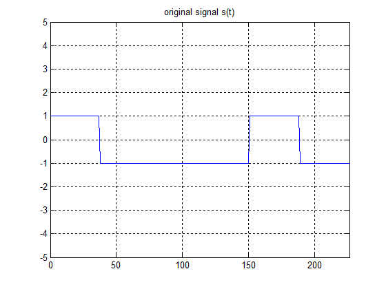
MATLAB code with comments for explanation is given below in bold letters, followed by the results.

clc;
close all;
clear all;

% define time T
T = 12*pi;

% frequency of square wave
f = 1/(4*T);

% define the sampling time
fs = 1;

% define time t
t = 0:1/fs:10*T;

% percentage Duty cycle
D =25;

% define the signal s(t)
s = square(2*pi*f*t,D);

% plot the signal
figure;
plot(t,s);grid on;ylim([-5 5]);xlim([0 6*T]);
title('original signal s(t)');

% now define the noise
AWGN= rand(size(s));

Att=(1);
nSig= Att*AWGN;

% add the noise to signal
y=s+nSig; %Square wave signal with Gaussian noise

% plot the noise contaminated signal
figure;
plot(t,y);grid on;ylim([-5 5]);xlim([0 6*T]);
title('noisy signal y(t)');

% take the fft of the original signal
% Finding FFT of s(t)
N = nextpow2(length(s));
S = fftshift(fft(s,2^N));
S = 2*S/length(s);
k = -(length(S)-1)/2:1:length(S)/2;
f = k/length(S) * fs;
figure;plot(f,abs(S));grid;
xlabel('Frequency in Hz');
ylabel('Amplitude');
title('Double sided Magnitude spectrum of original signal s(t)');
xlim([-1 1]);

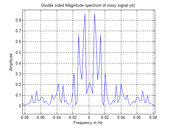
% take the fft of the noise contaminated signal
% Finding FFT of y(t)
N = nextpow2(length(y));
Y = fftshift(fft(y,2^N));
Y = 2*Y/ length(y);
k = -(length(Y)-1)/2:1:length(Y)/2;
f = k/length(Y) * fs;
figure;plot(f,abs(Y));grid;
xlabel('Frequency in Hz');
ylabel('Amplitude');
title('Double sided Magnitude spectrum of noisy signal y(t)');
xlim([-1 1]);

original signal s(t) LO 4 3 2 1 0 -1 N -3 -4 -5 50 100 150 200

noisy signal y(t) 5 4 3 2 www 0 Wwwwwwwwwwww MA -1 N -3 -4 -5 50 100 150 200

Double sided Magnitude spectrum of original signal s(t) 0.9 0.8 0.7 0.6 0.5 Amplitude 0.4 0.3 0.2 0.1 m What -0.08 -0.06 -0.04 0 0.04 0.06 0.08 -0.02 0.02 Frequency in Hz

Double sided Magnitude spectrum of noisy signal y(t) 0.8 0.7 0.6 0.5 Amplitude 0.4 0.3 0.2 0.1 White -0.08 -0.06 -0.04 0.04 0.06 0.08 -0.02 0 0.02 Frequency in Hz

Double sided Magnitude spectrum of noisy signal y(t) 0.8 0.7 0.6 0.5 Amplitude 0.4 0.3 0.2 0.1 White -0.08 -0.06 -0.04 0.04 0.06 0.08 -0.02 0 0.02 Frequency in Hz