Question

Homework 5 (35 Points max) Please Submit all Matlab and Data files that you create for this homework Problem 1 (max 20 Points): For the second-order drag model (see Eq.(1)), compute the velocity of a free-falling parachutist using Euler's method for the case where m80 kg and cd 0.25 kg/m. Perform the calculation from t 0 to 20 s with a step size of 1ms. Use an initial condition that the parachutist has an upward velocity of 20 m/s at t0. At t 10 s, assume that the chute is instantaneously deployed so that the drag coefficient jumps to 15 kg/m. Plot the velocity vs. time. This is a Matlab task. Solve this problem using a single for-loop and no more than two if-statements Grading Matrix for Problem 1 (max 20 Points in total): (a) up to 4 Points, if a for loop has been used for to increment the time. (b)up to 4 Points, if an if-statement has been used for the selection of the correct ca value. different physical cases (direction of drag, and direction of velocity) (velocity vs time). (c) up to 6 Points, if an if-statement has been used to differentiate the 3 (d) up to 6 Points, if the velocity data is correct and plotted in plotted correctly Problem 2 (max 15 Points): The following data for the density of water versus temperature comes from a table that was measured with high precision Solve this problem by using the Matlab functions polyfit and polyval. Please note, that you can use only polyval to evaluate any polynomial (a) Fit a third-order polynomial to the data. To ensure high numerical stability, use the scaling (b) Plot the polynomial estimated in (a) using 1000 samples where T is in the interval [0, 16] (blue (c) Determine an inverse polynomial to estimate the temperature corresponding to a density of capabilities of polyfit. line). Plot the raw data as well on top of that plot (red dots, not connected). 0.9993 g/cm2. Base your estimate on a third-order interpolating polynomial and assume T> 4 C. Determine with the help of the Newton-Raphson method the temperature T that corresponds to a density of 0.9993 g/cm2.Estimate a new polynomial but do not use any scaling features of polyfit. Use the coefficients obtained via polyfit to estimate the coefficients of the derivative. (d) (e) Compare the results in (c) and (d). Leave a comment in your Matlab code that discusses the difference in the results. 12 16 Density 0.99987 0.99988 0.99952 0.99897

Answer 1

Kindly upload different questions separately. Thank you!

Please rate the answer. Thank you!

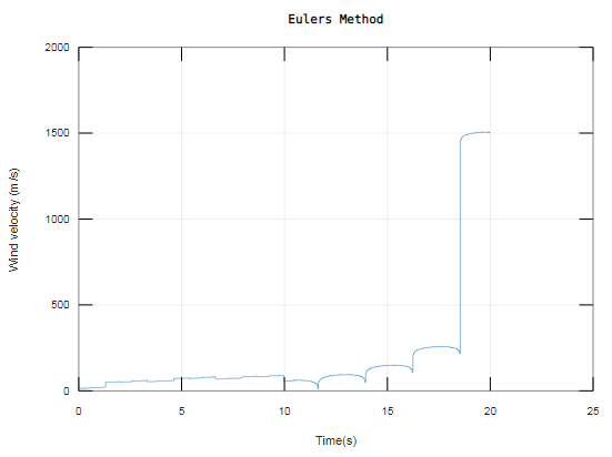
MATLAB Code:

m=80;
c1=0.25;
c2=1.5;
g=9.81;
t(1)=0;
v(1)=20;
h=0.001; &Step size
for i=1:20000
if i<10000
m=g-(c1/m)*v0*v0;
end
if i>=10000
m=g-(c2/m)*v0*v0;
end
v(i+1)=v(i)+h*m;
t(i+1)=t(i)+h;
end

plot(t,v)
xlabel('Time(s)')
ylabel('Wind velocity (m/s)')
title('Eulers Method')
grid on

Result:

Eulers Method 2000 1500 500_ 5i 15 20 25 Time(s)